How Many Units Will We Use?
A regression model that predicts a home's summer electricity from what is in it — and shows exactly what each hour of AC costs.
1Introduction
In summer the electricity bill jumps, and it arrives after the month is over. By then nothing can be done about it.
Families know roughly what they have — how many people, how many rooms, how many ACs and for how long. What they cannot do is turn that into a number of units before the month begins, or see which of those things costs the most.
This project builds a model that predicts a home's units for a summer month from five simple facts, and then uses what it learned to show how much one change would save.
Affordable and Clean Energy
Climate Action
SDG 7 asks for energy that is affordable, and for using it more efficiently. Most of India's electricity still comes from burning coal, so every unit saved is also less carbon dioxide — which is SDG 13. A family that can see its bill coming, and what drives it, can cut it.
The curriculum asks that the project be related to the Sustainable Development Goals. That link is the reason the problem is worth solving, so it belongs at the very start of the report, not tacked on at the end.
2Stage 1 — Problem Scoping
Problem scoping means understanding the problem properly before building anything. The tool for it is the 4Ws Problem Canvas: who has the problem, what the problem is, where it happens, and why solving it matters.
- Families paying the electricity bill
- Eco-clubs and electricity companies encouraging people to save power
- The summer bill is a surprise that comes too late to act on
- Families do not know which appliance costs them the most
- Homes in hot cities
- In the summer months, when ACs run for hours
- A family can plan and save before the bill arrives
- Saving electricity means burning less coal
The problem statement
The four answers are then joined into one sentence, using the curriculum's problem statement template:
Families who want to know their summer bill in advance, and an electricity company or school eco-club running an energy-saving campaign.
How it is done today
What most families do. The bill is exact, but it comes too late to change anything.
A rough guide. It does not change when the family buys a new AC or a new member joins.
Star labels give each appliance's power. Turning those into a monthly total means knowing how long each runs, which few people work out.
Objectives
- To read the summer electricity use of 400 homes from a CSV file
- To remove homes with no meter reading or impossible AC hours
- To find, with charts, which features push electricity use up
- To build three regression models and compare them
- To judge them with the curriculum's formulas for error and accuracy
- To predict units for new homes and work out what using less AC would save
📘 Revise: Stage 1 — Problem Scoping
3Stage 2 — Data Acquisition
Each row is one home: how many people live there, how many rooms, how many ACs, how many hours a day each AC runs, and whether there is an electric geyser. The last column is the units (kWh) on the meter for that summer month — the label.
The file has 400 rows.
For a real project, ask families in your colony to share last summer's bill and to answer five questions. A survey form works well. Use a home number, never a name or address, and tell people what the data is for.
Features and label
The features are what the model is given. The label is the answer it has to learn to give.
| Column | Type | What it holds | Role |
|---|---|---|---|
members | integer | People living in the home | feature |
rooms | integer | Number of rooms | feature |
ac_count | integer | Number of air conditioners | used to make ac_total_hours |
ac_hours | integer | Hours a day each AC runs | used to make ac_total_hours |
ac_total_hours | integer | ac_count × ac_hours — made by the program | feature |
geyser | 0 or 1 | 1 if the home has an electric geyser | feature |
units | integer | Units (kWh) used in the month — what the model must predict | label |
home_id | text | A home number, never an address | not used |
The first eight rows of home_energy.csv
| home_id | members | rooms | ac_count | ac_hours | geyser | units |
|---|---|---|---|---|---|---|
H301 | 1 | 1 | 1 | 4 | 0 | 233 |
H302 | 6 | 3 | 0 | 0 | 1 | 242 |
H303 | 5 | 4 | 3 | 10 | 0 | 1129 |
H304 | 4 | 3 | 1 | 10 | 0 | 483 |
H305 | 6 | 3 | 3 | 5 | 1 | 697 |
H306 | 2 | 1 | 0 | 0 | 0 | 76 |
H307 | 7 | 4 | 0 | 0 | 1 | 262 |
H308 | 3 | 2 | 3 | 8 | 1 | 918 |
Inside home_energy.csv
Four hundred homes and their units in one summer month. A few meter readings are blank, and two homes have AC hours typed wrongly. The whole file is 400 rows, 7.5 KB. It comes with the project download, and you can take the file on its own.
📘 Revise: Stage 2 — Data Acquisition
4Stage 3 — Data Exploration
Data exploration means getting to know the data before trusting it: fixing what is wrong with it, then drawing it to see the patterns. The charts here are what decide what the model should be.
What was wrong with the data
A home with no units cannot teach the model anything, so it is removed and counted.
A day has 24 hours, so 60 or 80 hours is a typing mistake (6 or 8 with an extra 0). Guessing which it was would be inventing data, so those homes are removed.
Two ACs for 5 hours use about as much as one AC for 10. So the program makes one new feature, ac_total_hours = ac_count × ac_hours. Making a better feature from the ones you have is part of data exploration.
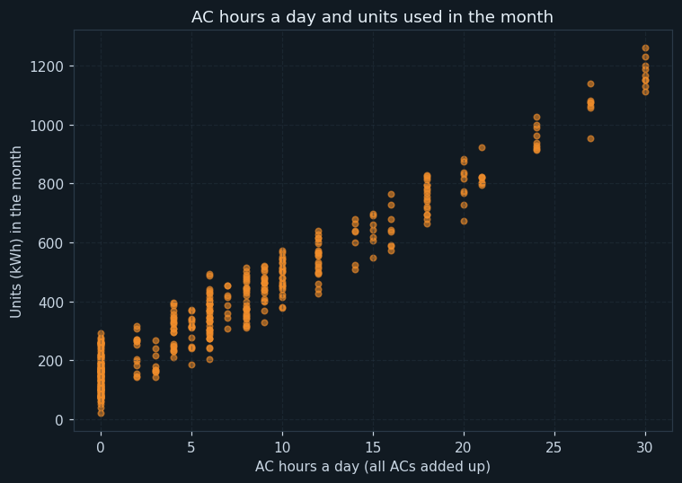
Each dot is one home: AC hours a day across, units in the month up.
The dots climb in a clear straight band. The more AC hours, the more units, and by about the same amount for every extra hour. A straight-line pattern like this is what a regression model is built to find.
The band is wide, though. At 0 AC hours, homes still use anything from about 20 to 300 units. Something other than the AC is making the difference — the next chart looks at one of those things.
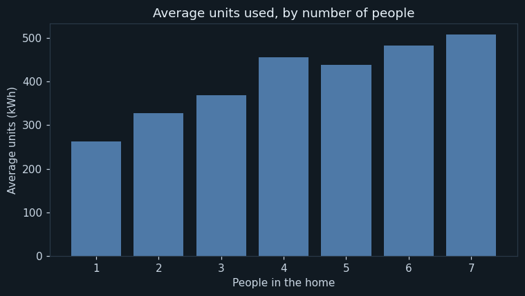
One bar for each family size. The height is the average units those homes used.
Bigger families use more — more lights, more fans, more washing. The bars do not rise perfectly evenly because family size is mixed up with how many ACs a home has. A model that looks at every feature together can separate the two; one chart cannot.
📘 Revise: Stage 3 — Data Exploration
5Stage 4 — Modelling
Where this model sits in the family of AI models:
The answer is a number — how many units — not a group. Predicting a number is regression. The training homes come with their real units, so it is supervised learning.
How the model works
The homes are split into 316 for training and 79 for testing. Three models are built from the training homes.
Model A always guesses the average of the training homes. It is not meant to be good — it is the baseline every real model must beat.
Model B draws the straight line that best fits AC hours and units. The program found it to be: units = 149.3 + 33.3 x AC hours a day.
Model C uses all four features. It works out units as a weighted sum: each feature is multiplied by a weight, the results are added, and a bias is added on top. This is the same sum a perceptron does in Unit 2 — inputs times weights, plus a bias. The difference is that here the computer finds the weights itself, choosing the ones that make its predictions for the training homes as close as possible to the real meter readings.
The weights it learned can be read like a price list: every AC hour a day adds about 32 units to the month, every person about 20, and a geyser about 38.
📘 Revise: Stage 4 — Modelling
6Stage 5 — Evaluation
A regression model is judged by how far off its predictions are. The curriculum's formulas were used for every testing home: error = |actual − predicted|, error rate = error ÷ actual, and accuracy = 1 − error rate. The model's accuracy is the average of all those accuracies.
Model C was off by 20.1 units on average, an accuracy of 92.1 %.
Model A's accuracy is very low, and the reason is worth knowing. For a small home that uses 60 units, guessing the average of about 400 gives an error of 340 — more than five times the actual. The error rate is then above 1, and the accuracy for that home is negative. When those are averaged in, the total falls sharply. Dividing by the actual value punishes big mistakes on small homes, which is exactly what the formula is meant to do.
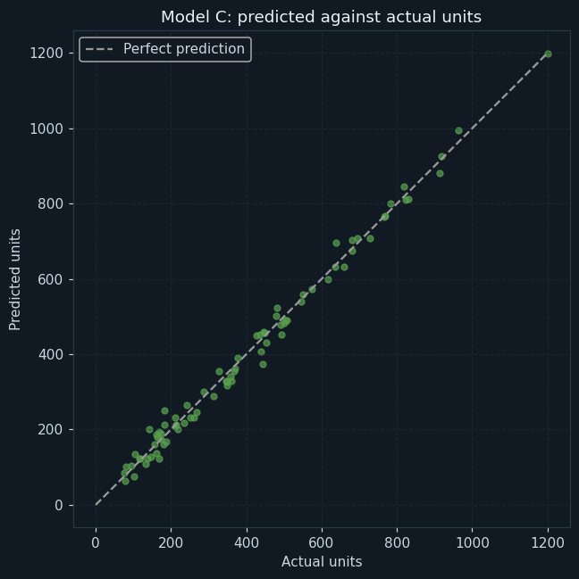
Each dot is one testing home: its real units across, the model's prediction up. A perfect model would put every dot on the dashed line.
The dots hug the line from the smallest homes to the largest. The model is not just right on average; it is right for small and large homes alike.
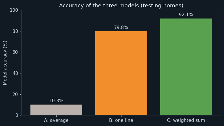
One bar per model: its accuracy on the testing homes, worked out with the curriculum's formula.
Guessing the average scores only 10.3 %. That shows why a baseline is worth having: it is what a model has to beat. One line through AC hours reaches 79.8 %, and using every feature reaches 92.1 %.
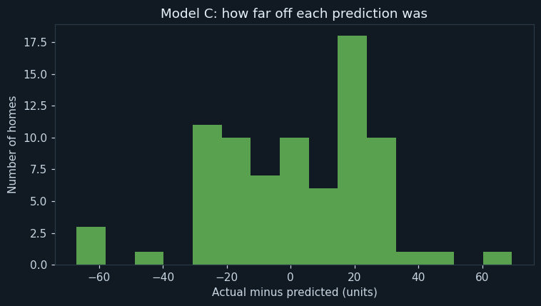
Each bar counts testing homes whose prediction was off by that much. Left of zero, the model guessed too high; right of zero, too low.
Most predictions are within about 30 units, and the mistakes are spread on both sides of zero. The model does not always guess too high or always too low, which means it is not biased in one direction.
📘 Revise: The Confusion Matrix
7Stage 6 — Deployment
The program predicts the units for three new homes. It then asks a question a family actually cares about: what if the first home ran its AC two hours a day less? The answer, 64 units a month for the first home, comes straight from the weight the model learned for AC hours.
In real use, a family would type in its five facts at the start of summer and see the month's units — and then try changes, such as fewer AC hours or setting the AC to 24°C, to see what each would save.
📘 Revise: Stage 6 — Deployment
8Ethical concerns
An AI project is not finished when the model works. The curriculum asks three questions of every model — is it fair (bias), can it explain itself (transparency), and who answers for its mistakes (accountability). For this project:
This model can explain itself completely: four weights and a bias, printed in the output. A family can see exactly why it predicts what it does. That makes it easy to trust and easy to check.
The homes are from one hot city in one summer month. In a cooler city, or in winter, the same home would use far less. The model should not be used outside the conditions it learned from.
An electricity bill shows when a family is at home and how they live. Data must be shared willingly, stored with a home number only, and never published with addresses.
📘 Revise: Bias, Transparency, Accountability
9Source code
The whole program — it is also in the downloads at the top of this page — in Python with pandas, NumPy and matplotlib — the three libraries of Unit 7. It is laid out as the six stages of the AI Project Cycle, one after another. Every chart on this page was drawn by it, and every number came out of running it.
# ---------------------------------------------------------------------------
# home_energy.py
#
# AI project on Statistical Data: predicting how many units of electricity a
# home will use in a summer month, from what is in the home.
#
# CBSE Class X, Artificial Intelligence (417), Part C project work.
# SDG 7 (Affordable and Clean Energy) and SDG 13 (Climate Action).
#
# This is a REGRESSION project: the answer is a number, not a group. Three
# models are compared, each a little cleverer than the last:
#   A. always guess the average home
#   B. a line of best fit through one feature (AC hours a day)
#   C. a weighted sum of every feature - each feature times a weight, plus a
#      bias, the same sum a perceptron works out in Unit 2
#
# They are judged the way the curriculum judges a regression model:
#   error = |actual - predicted|,  error rate = error / actual,
#   accuracy = 1 - error rate,  model accuracy = mean of all the accuracies.
#
# Libraries: pandas (the data), numpy (the arithmetic), matplotlib (charts).
# ---------------------------------------------------------------------------

# %% Stage 1 - Problem scoping
print("=" * 60)
print("HOW MANY UNITS WILL WE USE?")
print("=" * 60)
print("Who   : families paying the electricity bill")
print("What  : the summer bill arrives as a shock, too late to act")
print("Where : homes in a hot city, in the months the AC runs")
print("Why   : knowing in advance helps a family save power")
print()

# %% Stage 2 - Data acquisition
import pandas as pd
import numpy as np
import matplotlib.pyplot as plt

pd.set_option("display.width", 120)
pd.set_option("display.max_columns", 20)

data = pd.read_csv("home_energy.csv")

print("--- Stage 2: Data acquisition ---")
print("Rows read    :", len(data))
print("Columns read :", len(data.columns))
print()
print("The first 10 rows:")
print(data.head(10))
print()

# %% Stage 3 - Data exploration
print("--- Stage 3: Data exploration ---")

# A home with no meter reading cannot teach the model anything.
missing = data["units"].isnull().sum()
data = data.dropna(subset=["units"])
print("Rows with no meter reading       :", missing, "(removed)")

# A day has 24 hours, so 60 or 80 AC hours a day is a typing mistake.
impossible = (data["ac_hours"] > 24).sum()
data = data[data["ac_hours"] <= 24]
print("Rows with more than 24 AC hours  :", impossible, "(removed)")
print("Rows left                        :", len(data))
print()

# One new feature, made from two: how many AC-hours the home runs in a day.
# Two ACs for 5 hours use about as much power as one AC for 10.
data["ac_total_hours"] = data["ac_count"] * data["ac_hours"]

units = data["units"]
print("Units in a month - mean   :", round(np.mean(units), 1))
print("Units in a month - median :", np.median(units))
print("Units in a month - lowest :", units.min(), " highest :", units.max())
print()

by_members = data.groupby("members")["units"].mean().round(1)
print("Average units, by number of people in the home:")
print(by_members)
print()

# Chart 1: AC hours a day against units.
plt.figure(figsize=(7, 5))
plt.scatter(data["ac_total_hours"], data["units"], alpha=0.6, s=18, color="#f28e2b")
plt.title("AC hours a day and units used in the month")
plt.xlabel("AC hours a day (all ACs added up)")
plt.ylabel("Units (kWh) in the month")
plt.grid(True, linestyle="--", alpha=0.4)
plt.tight_layout()
plt.savefig("chart1_ac_hours.png")
plt.close()

# Chart 2: average units by family size.
plt.figure(figsize=(7, 4))
plt.bar(by_members.index, by_members.values, color="#4e79a7")
plt.title("Average units used, by number of people")
plt.xlabel("People in the home")
plt.ylabel("Average units (kWh)")
plt.tight_layout()
plt.savefig("chart2_members.png")
plt.close()

# %% Stage 4 - Modelling
print("--- Stage 4: Modelling ---")

features = ["members", "rooms", "ac_total_hours", "geyser"]
label = "units"

data = data.sample(frac=1, random_state=5)
cut = int(len(data) * 0.8)
train = data[:cut]
test = data[cut:]
print("Training rows :", len(train))
print("Testing rows  :", len(test))
print()

# Model A: always guess the average of the training homes.
average = train[label].mean()
predict_a = np.full(len(test), average)
print("Model A guesses every home will use", round(average, 1), "units")

# Model B: the straight line that fits AC hours and units best.
# np.polyfit with 1 finds the slope and the starting point of that line.
slope, start = np.polyfit(train["ac_total_hours"], train[label], 1)
predict_b = slope * test["ac_total_hours"] + start
print("Model B line : units =", round(start, 1), "+", round(slope, 1), "x AC hours a day")

# Model C: a weighted sum of all four features, plus a bias.
#     units = bias + w1 x members + w2 x rooms + w3 x AC hours + w4 x geyser
# np.linalg.lstsq finds the weights that make the predictions on the
# training homes as close as possible to the real units. The column of 1s
# is what lets it find the bias, exactly like the bias input of a perceptron.
X_train = train[features].copy()
X_train["bias"] = 1
weights = np.linalg.lstsq(X_train.values, train[label].values.astype(float), rcond=None)[0]

print()
print("What model C learned (one weight for each feature):")
for i in range(len(features)):
    print("  " + features[i].ljust(16), round(weights[i], 1))
print("  " + "bias".ljust(16), round(weights[4], 1))
print()

X_test = test[features].copy()
X_test["bias"] = 1
predict_c = X_test.values.dot(weights)

# %% Stage 5 - Evaluation
print("--- Stage 5: Evaluation ---")
actual = test[label].values.astype(float)

names = ["A: average", "B: one line", "C: weighted sum"]
model_accuracy = []
mean_error = []
for predicted in [predict_a, predict_b, predict_c]:
    error = np.abs(actual - predicted)          # error = |actual - predicted|
    error_rate = error / actual                 # error rate = error / actual
    accuracy = 1 - error_rate                   # accuracy = 1 - error rate
    model_accuracy.append(np.mean(accuracy) * 100)
    mean_error.append(np.mean(error))

for i in range(3):
    print("Model " + names[i].ljust(16), "average error :", str(round(mean_error[i], 1)).rjust(6),
          "units   accuracy :", round(model_accuracy[i], 1), "%")
print()
print("Average error of model C :", round(mean_error[2], 1), "units")
print("Accuracy of model C      :", round(model_accuracy[2], 1), "%")
print("Accuracy of model B      :", round(model_accuracy[1], 1), "%")
print("Accuracy of model A      :", round(model_accuracy[0], 1), "%")
print()

# Chart 3: model C's predictions against the real units.
plt.figure(figsize=(6, 6))
plt.scatter(actual, predict_c, alpha=0.7, s=20, color="#59a14f")
top = max(actual.max(), predict_c.max())
plt.plot([0, top], [0, top], color="#999999", linestyle="--", label="Perfect prediction")
plt.title("Model C: predicted against actual units")
plt.xlabel("Actual units")
plt.ylabel("Predicted units")
plt.legend()
plt.grid(True, linestyle="--", alpha=0.4)
plt.tight_layout()
plt.savefig("chart3_predicted_actual.png")
plt.close()

# Chart 4: the three models compared.
plt.figure(figsize=(7, 4))
plt.bar(names, model_accuracy, color=["#bab0ac", "#f28e2b", "#59a14f"])
plt.ylim(0, 100)
plt.title("Accuracy of the three models (testing homes)")
plt.ylabel("Model accuracy (%)")
for i in range(3):
    plt.text(i, model_accuracy[i] + 2, str(round(model_accuracy[i], 1)) + "%", ha="center")
plt.tight_layout()
plt.savefig("chart4_models.png")
plt.close()

# Chart 5: how far off each testing home was, for model C.
plt.figure(figsize=(7, 4))
plt.hist(actual - predict_c, bins=15, color="#59a14f")
plt.title("Model C: how far off each prediction was")
plt.xlabel("Actual minus predicted (units)")
plt.ylabel("Number of homes")
plt.tight_layout()
plt.savefig("chart5_errors.png")
plt.close()

# %% Stage 6 - Deployment
print("--- Stage 6: Deployment ---")
homes = pd.DataFrame({
    "members":        [4, 2, 6],
    "rooms":          [3, 1, 4],
    "ac_total_hours": [16, 0, 24],
    "geyser":         [1, 0, 1],
})
homes["bias"] = 1
forecast = homes.values.dot(weights)
for i in range(len(homes)):
    h = homes.iloc[i]
    print("People", h["members"], " rooms", h["rooms"], " AC hours a day", h["ac_total_hours"],
          " geyser", h["geyser"], "->", round(forecast[i]), "units")

# What would two hours less AC a day save the first home?
fewer = homes.iloc[[0]].copy()
fewer["ac_total_hours"] = fewer["ac_total_hours"] - 2
saving = forecast[0] - fewer.values.dot(weights)[0]
print("Saving from two AC hours a day less :", round(saving), "units a month for the first home")
The library calls it is built from
| Call | Where | What it does |
|---|---|---|
pd.read_csv() | Stage 2 | Reads the CSV file |
dropna(subset=["units"]) | Stage 3 | Removes homes with no meter reading |
data[data["ac_hours"] <= 24] | Stage 3 | Keeps only possible AC hours |
data["ac_count"] * data["ac_hours"] | Stage 3 | Makes the new feature ac_total_hours |
plt.scatter / plt.bar / plt.hist | Stages 3, 5 | Scatter plots, bar charts and a histogram |
np.polyfit(x, y, 1) | Stage 4 | Finds the straight line that fits best (model B) |
np.linalg.lstsq() | Stage 4 | Finds the weights and bias of the weighted sum (model C) |
.dot(weights) | Stage 4 | Multiplies each feature by its weight and adds them up |
np.abs(actual - predicted) | Stage 5 | The error for every testing home |
np.mean() | Stage 5 | The average accuracy and the average error |
10Sample output
A real run, exactly as it appeared. Nothing below was typed by hand.
============================================================
HOW MANY UNITS WILL WE USE?
============================================================
Who   : families paying the electricity bill
What  : the summer bill arrives as a shock, too late to act
Where : homes in a hot city, in the months the AC runs
Why   : knowing in advance helps a family save power

--- Stage 2: Data acquisition ---
Rows read    : 400
Columns read : 7

The first 10 rows:
  home_id  members  rooms  ac_count  ac_hours  geyser   units
0    H301        1      1         1         4       0   233.0
1    H302        6      3         0         0       1   242.0
2    H303        5      4         3        10       0  1129.0
3    H304        4      3         1        10       0   483.0
4    H305        6      3         3         5       1   697.0
5    H306        2      1         0         0       0    76.0
6    H307        7      4         0         0       1   262.0
7    H308        3      2         3         8       1   918.0
8    H309        7      5         3        10       0  1200.0
9    H310        3      1         0         0       0   131.0

--- Stage 3: Data exploration ---
Rows with no meter reading       : 3 (removed)
Rows with more than 24 AC hours  : 2 (removed)
Rows left                        : 395

Units in a month - mean   : 407.3
Units in a month - median : 350.0
Units in a month - lowest : 22.0  highest : 1260.0

Average units, by number of people in the home:
members
1    262.9
2    327.6
3    368.7
4    454.7
5    436.9
6    481.9
7    506.8
Name: units, dtype: float64

--- Stage 4: Modelling ---
Training rows : 316
Testing rows  : 79

Model A guesses every home will use 409.0 units
Model B line : units = 149.3 + 33.3 x AC hours a day

What model C learned (one weight for each feature):
  members          20.1
  rooms            12.0
  ac_total_hours   32.2
  geyser           37.7
  bias             31.9

--- Stage 5: Evaluation ---
Model A: average       average error :  211.5 units   accuracy : 10.3 %
Model B: one line      average error :   51.5 units   accuracy : 79.8 %
Model C: weighted sum  average error :   20.1 units   accuracy : 92.1 %

Average error of model C : 20.1 units
Accuracy of model C      : 92.1 %
Accuracy of model B      : 79.8 %
Accuracy of model A      : 10.3 %

--- Stage 6: Deployment ---
People 4  rooms 3  AC hours a day 16  geyser 1 -> 702 units
People 2  rooms 1  AC hours a day 0  geyser 0 -> 84 units
People 6  rooms 4  AC hours a day 24  geyser 1 -> 1012 units
Saving from two AC hours a day less : 64 units a month for the first home11The same project without code
Orange's Linear Regression widget builds the same weighted-sum model, and Test and Score reports the average error. The tool is Orange Data Mining.
Load home_energy.csv. Set units as the target and home_id as a meta attribute.
Keep rows where ac_hours is at most 24; remove rows with units missing.
Make ac_total_hours = ac_count * ac_hours.
Plot ac_total_hours against units — the same as chart 1.
Keep 80% for training; the remaining 20% is for testing.
The weighted-sum model (model C).
Test on the testing data. For regression it reports errors such as MAE, the mean absolute error — the same as this program's average error.
Connect the coefficients output to a Data Table to see the learned weights.
📘 Revise: No-Code AI, and Orange
12Testing
Every case below was actually run, and the result is what came back. Each one gives the whole program a small input of its own.
| Test case | Expected | Actual | Result |
|---|---|---|---|
| The full dataset | Rows read : 400 | Rows read : 400 | Pass |
| Homes with no meter reading are removed | Rows with no meter reading : 3 (removed) | Rows with no meter reading : 3 (removed) | Pass |
| 80 and 60 AC hours a day are impossible, so removed | Rows with more than 24 AC hours : 2 (removed) | Rows with more than 24 AC hours : 2 (removed) | Pass |
| The weighted sum beats the single line | Accuracy of model C : 92.1 % | Accuracy of model C : 92.1 % | Pass |
| Units that follow an exact rule: model C finds it and is never wrong | Accuracy of model C : 100.0 % | Accuracy of model C : 100.0 % | Pass |
| ...and learns the rule's own weight for AC hours | ac_total_hours 30.0 | ac_total_hours 30.0 | Pass |
| Boundary: 24 AC hours a day is kept, 25 is removed | Rows with more than 24 AC hours : 1 (removed) | Rows with more than 24 AC hours : 1 (removed) | Pass |
| The data file is missing | FileNotFoundError: [Errno 2] No such file or directory: 'home_energy.csv' | FileNotFoundError: [Errno 2] No such file or directory: 'home_energy.csv' | Pass |
13Results, limits and what next
- Model C, a weighted sum of four features, predicts a home's summer units with an accuracy of 92.1 %.
- AC hours are the biggest driver: each AC hour a day adds about 32 units to the month.
- One feature on its own (model B) reaches 79.8 %; using every feature together does much better.
- Guessing the average scores only 10.3 % — the baseline that shows the model is really learning.
- Two hours less AC a day would save a typical home about 64 units a month.
What this model cannot do
- One summer month in one city; it says nothing about winter or a cooler place
- It does not know how efficient each AC is (its star rating) or what temperature it is set to
- It predicts units, not the bill — electricity tariffs differ from state to state
- It treats every person and every room as using the same amount
What to add next
This is where you make the project your own. Take one of these, or an idea of yours:
- Add the AC's star rating and set temperature as features
- Collect bills for a whole year and add the month as a feature
- Convert the units into a bill using your own state's tariff
- Run an eco-club campaign: predict, ask families to cut AC hours, and compare the next bills
What you may have to learn on your own
- What regression is, and how it differs from classification
- The curriculum's error and accuracy formulas, and why accuracy can go negative for one prediction
- How a weighted sum with a bias is the same idea as the perceptron
- Making a new feature from existing ones (ac_count × ac_hours)
14Conclusion
A home's summer electricity can be predicted well from five simple facts. The weighted-sum model was off by about 20.1 units on average, an accuracy of 92.1 %.
The model is useful beyond its predictions. Because it is a weighted sum, its weights are a price list for the home: they show that the AC drives the bill far more than anything else, and they turn "use the AC less" into a number a family can act on.
Comparing three models was worth the effort. The baseline showed that the model really learned something, and the single line showed that one feature is not enough.
15Questions for the viva
The project carries a viva voce of its own, worth 5 marks. These are the questions it is most likely to ask about this project. Try answering each one aloud before opening it.
▸Is your project classification or regression? Why?
Regression, because the answer is a number of units, not a group.
▸How did you calculate the accuracy of a regression model?
For each testing home: error = |actual − predicted|, error rate = error ÷ actual, accuracy = 1 − error rate. The model accuracy is the average over all the homes.
▸Why did you build model A, which only guesses the average?
As a baseline. A real model must do better than simply guessing the average; otherwise it has learned nothing.
▸How is model C like a perceptron?
Both multiply each input by a weight, add them up and add a bias. Here the computer finds the weights from the training data.
▸What is ac_total_hours and why did you make it?
It is ac_count × ac_hours — the total AC hours a day. Two ACs for 5 hours use about as much as one for 10, so one feature describes it better than two.
▸Why did you remove homes with more than 24 AC hours?
A day only has 24 hours, so those values are typing mistakes.
▸Which SDGs does it relate to?
SDG 7, Affordable and Clean Energy, and SDG 13, Climate Action, because saving electricity means burning less coal.
16References
- Bureau of Energy Efficiency, Government of India, star labelling programme — https://beeindia.gov.in/
- Central Electricity Authority, energy statistics — https://cea.nic.in/
- Orange Data Mining, Linear Regression widget — https://orangedatamining.com/widget-catalog/model/linearregression/
- CBSE, Artificial Intelligence (Subject Code 417), Class X curriculum, 2026-27 — Part C, Practical and Project Work
- CBSE, Artificial Intelligence Facilitator Handbook, Class X
- pandas — https://pandas.pydata.org/docs/; NumPy — https://numpy.org/doc/; Matplotlib — https://matplotlib.org/stable/
- LambdaLab — https://www.lambdalab.in