Grouping Homes by Water Use
Clustering with no labels at all: k-means finds the careful, typical and heavy water users in a housing society by itself.
1Introduction
Every summer the society's tank runs low, and every summer the same notice goes up: "Please save water." Nobody reads it, because it speaks to everyone and so to no one.
The flats are not all the same. Some already use little. Some water a garden for half an hour a day. Some wash a car every other day. Each needs different advice.
But nobody has sorted the flats into groups, and there is no column saying who is careful and who is not. This project asks the computer to find those groups on its own.
Clean Water and Sanitation
Sustainable Cities and Communities
SDG 6 asks for water to be used efficiently, and many Indian cities run short every summer. A housing society that knows which homes use the most water, and why, can give each group advice that fits — and save far more than a single notice on the board ever does.
The curriculum asks that the project be related to the Sustainable Development Goals. That link is the reason the problem is worth solving, so it belongs at the very start of the report, not tacked on at the end.
2Stage 1 — Problem Scoping
Problem scoping means understanding the problem properly before building anything. The tool for it is the 4Ws Problem Canvas: who has the problem, what the problem is, where it happens, and why solving it matters.
- The society's water committee
- Every family in the society, who share one tank
- Water runs short every summer
- One general notice does not change anybody's habits
- A housing society with a water meter in every flat
- In the summer months
- Advice that fits a household is more likely to be followed
- Saving water keeps the tank from running dry
The problem statement
The four answers are then joined into one sentence, using the curriculum's problem statement template:
The water committee of a housing society with a meter in every flat, or a municipal water department planning a saving campaign.
How it is done today
Cheap and quick, and almost always ignored, because it is written for everyone at once.
Some societies split the bill by meter. It tells a family how much they used, but not whether that is a lot, or what to change.
For example, "no garden watering after 8 am". Useful, but the committee has to guess which habits matter most.
Objectives
- To read a month of water-meter data for 300 flats from a CSV file
- To remove blank and impossible (negative) meter readings
- To compare the society's use with the city norm of 135 litres a person a day
- To find groups of similar flats with k-means clustering, without any labels
- To check how many groups is the right number, and whether the groups are stable
- To place new flats into a group and suggest a tip for each
📘 Revise: Stage 1 — Problem Scoping
3Stage 2 — Data Acquisition
Each row is one flat: the litres used per person per day over the month (from the meter, divided by the number of people), the minutes a day the garden is watered, and the car washes in a week. There is no label — no column says which group a flat belongs to.
The file has 300 rows.
For a real project, ask the society office for a month of meter readings and send a short form to every flat asking about gardens and cars. Use flat numbers only, and get the committee's permission first.
Features and label
The features are what the model is given. The label is the answer it has to learn to give.
| Column | Type | What it holds | Role |
|---|---|---|---|
litres_per_person | integer | Litres used per person per day, from the meter | feature |
garden_minutes | integer | Minutes a day the garden or plants are watered | feature |
car_washes_week | integer | Car or scooter washes in a week | feature |
flat_no | text | Flat number, never a name | not used |
The first eight rows of water_use.csv
| flat_no | litres_per_person | garden_minutes | car_washes_week |
|---|---|---|---|
F101 | 91 | 9 | 2 |
F102 | 196 | 39 | 4 |
F103 | 234 | 36 | 4 |
F104 | 146 | 10 | 1 |
F105 | 136 | 9 | 2 |
F106 | 131 | 9 | 1 |
F107 | 103 | 4 | 0 |
F108 | 91 | 4 | 0 |
Inside water_use.csv
Three hundred flats and one month of water use. There is no label column. Some meter readings are blank and two are negative. The whole file is 300 rows, 3.9 KB. It comes with the project download, and you can take the file on its own.
📘 Revise: Stage 2 — Data Acquisition
4Stage 3 — Data Exploration
Data exploration means getting to know the data before trusting it: fixing what is wrong with it, then drawing it to see the patterns. The charts here are what decide what the model should be.
What was wrong with the data
A flat with no reading cannot be grouped, so it is removed and counted.
Water used cannot be less than zero. A negative number means the meter was reset in the middle of the month, so the reading is wrong and is removed. A reading of exactly 0 is kept — the flat may have been empty.
Each feature is rescaled to run from 0 to 1, so litres do not decide the groups on their own.
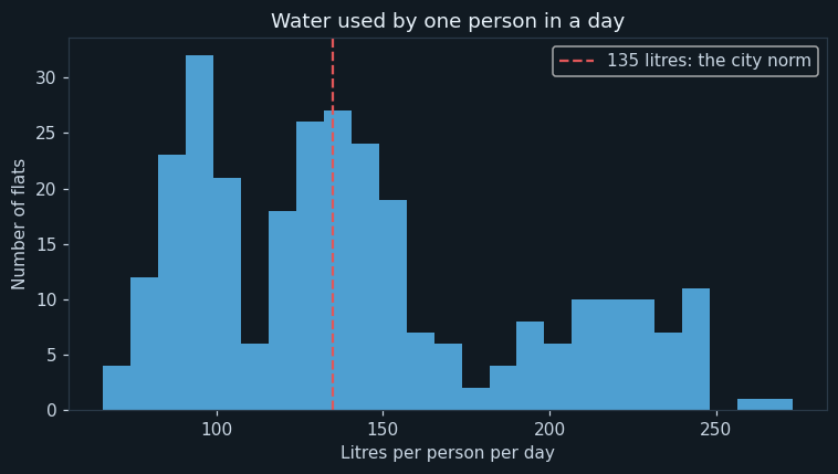
Each bar counts the flats in a range of litres per person per day. The red dashed line is 135 litres, the amount city planners use for one person in a day.
145 of 295 flats are above the norm. The histogram is not one smooth hill — there is a separate bump on the right, around 200 litres. A bump like that is a sign that the data holds more than one kind of household.
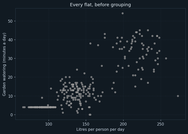
Each dot is one flat: litres per person across, garden minutes up. All the dots are grey because there are no labels.
Even in grey, the dots are not spread evenly. There is a crowd at the bottom left, another in the middle, and a looser group at the top right. Our eyes see groups — the question is whether the computer finds the same ones.
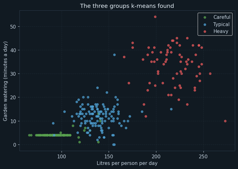
The same scatter plot, now coloured by the group each flat was put in.
The computer found the three crowds. Careful flats use about 96 litres a person and hardly water a garden. Typical flats use about 139. Heavy flats use about 217 litres and water a garden for over half an hour a day — the garden is a large part of why they are heavy.
The names Careful, Typical and Heavy were given by the program after the groups were found, by sorting them by average litres. K-means itself only says group 0, 1 and 2. Giving the groups meaning is a person's job.
📘 Revise: Stage 3 — Data Exploration
5Stage 4 — Modelling
Where this model sits in the family of AI models:
There is no label: no column says who is careful and who is heavy. When a model has to find patterns in data without being told the answers, it is unsupervised learning. Finding groups of similar items is clustering.
How the model works
The model is k-means, with k = 3 groups. It works in four steps. One: pick three flats at random as the first group centres. Two: put every flat in the group whose centre is nearest. Three: move each centre to the middle (the average) of the flats in its group. Four: repeat steps two and three until the groups stop changing.
K-means has one known weakness, and the program shows it. If two of the random first centres happen to land in the same crowd, it can get stuck with a poor grouping. In this run, one of the five starts got stuck. So the program runs k-means from 5 different random starts and keeps the grouping with the smallest spread — 4 of 5 starts found that same best grouping. Orange's k-Means widget does exactly this, and calls it re-runs.
📘 Revise: Stage 4 — Modelling
6Stage 5 — Evaluation
An unsupervised model cannot have an accuracy, because there are no right answers to compare with. It has to be judged in other ways, and this project uses two.
First, is 3 the right number of groups? The elbow chart answers that: the spread falls a lot up to k = 3 and only a little after it.
Second, are the groups real, or did the computer invent them? If they are real, k-means should find the same groups from different random starts. Four of the five starts ended with exactly the same grouping, and the fifth got stuck in a clearly worse one (a larger spread). That is strong evidence the three groups are really in the data.
Finally, a person has to check that the groups make sense. Here they do: each group has a clear story — careful users, typical users, and users with a garden and a car to wash.
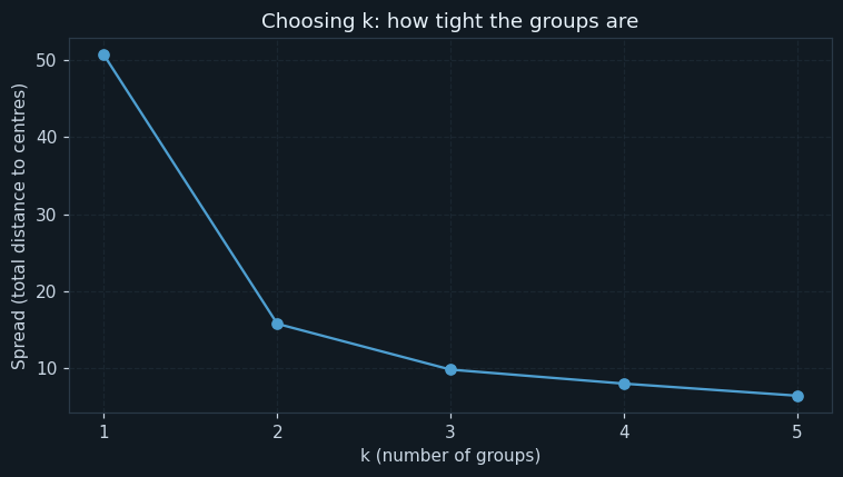
Across is k, the number of groups. Up is the spread: the total distance from every flat to the centre of its group. Lower means tighter groups.
Going from 2 groups to 3 cuts the spread by 5.94. Going from 3 to 4 cuts it by only 1.82. The line bends — like an elbow — at k = 3. After that, extra groups only split real groups into smaller pieces. So 3 is the right number.
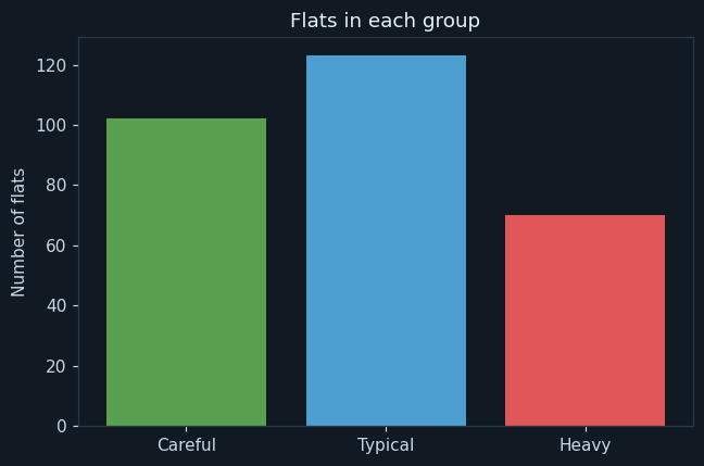
One bar per group: how many flats are in it.
The heavy group is the smallest, at about a quarter of the society. That is useful: the committee can talk to 70 households about gardens and cars instead of 295 about everything.
📘 Revise: The Confusion Matrix
7Stage 6 — Deployment
When a new family moves in, its first month of readings is placed in the group whose centre is nearest, and the program prints the tip for that group: a thank-you for careful users, help with taps for typical users, and garden and car advice for heavy users.
In real use the committee would run this every month and send each group its own message. Next summer, running it again would show whether flats have moved from the heavy group to the typical one.
📘 Revise: Stage 6 — Deployment
8Ethical concerns
An AI project is not finished when the model works. The curriculum asks three questions of every model — is it fair (bias), can it explain itself (transparency), and who answers for its mistakes (accountability). For this project:
"Heavy" is a description of water use, not a judgement of a family. A large family or someone who is unwell may need more water. Messages to each group should be helpful and private, never a list on the notice board.
Water use shows when a family is at home. Readings should be stored with flat numbers, seen only by the committee, and used only for saving water.
The groups are explained by their averages, which anyone can read. A family can see why it was put in a group.
📘 Revise: Bias, Transparency, Accountability
9Source code
The whole program — it is also in the downloads at the top of this page — in Python with pandas, NumPy and matplotlib — the three libraries of Unit 7. It is laid out as the six stages of the AI Project Cycle, one after another. Every chart on this page was drawn by it, and every number came out of running it.
# ---------------------------------------------------------------------------
# water_groups.py
#
# AI project on Statistical Data: finding groups of households by how they
# use water, so that a housing society can give each group the right advice.
#
# CBSE Class X, Artificial Intelligence (417), Part C project work.
# SDG 6 (Clean Water and Sanitation) and SDG 11 (Sustainable Cities).
#
# This is UNSUPERVISED learning. Nobody has told the program which flats are
# careful and which are wasteful - there is no label column at all. The
# model, k-means clustering, finds the groups by itself:
#   1. pick k flats at random as the first group centres
#   2. put every flat in the group whose centre is nearest
#   3. move each centre to the middle (the mean) of its group
#   4. repeat steps 2 and 3 until nothing changes
#
# Libraries: pandas (the data), numpy (the arithmetic), matplotlib (charts).
# ---------------------------------------------------------------------------

# %% Stage 1 - Problem scoping
print("=" * 60)
print("GROUPING HOMES BY WATER USE")
print("=" * 60)
print("Who   : the housing society's water committee")
print("What  : one notice for everyone is ignored by everyone")
print("Where : a society with a water meter in every flat")
print("Why   : advice that fits each group saves more water")
print()

# %% Stage 2 - Data acquisition
import pandas as pd
import numpy as np
import matplotlib.pyplot as plt

pd.set_option("display.width", 120)
pd.set_option("display.max_columns", 20)

data = pd.read_csv("water_use.csv")

print("--- Stage 2: Data acquisition ---")
print("Rows read    :", len(data))
print("Columns read :", len(data.columns))
print()
print("The first 10 rows:")
print(data.head(10))
print()

# %% Stage 3 - Data exploration
print("--- Stage 3: Data exploration ---")
features = ["litres_per_person", "garden_minutes", "car_washes_week"]

missing = data["litres_per_person"].isnull().sum()
data = data.dropna(subset=["litres_per_person"])
print("Rows with no meter reading     :", missing, "(removed)")

# Water used cannot be negative; a negative number means the meter was reset.
negative = (data["litres_per_person"] < 0).sum()
data = data[data["litres_per_person"] >= 0]
print("Rows with negative litres      :", negative, "(removed)")
print("Rows left                      :", len(data))
print()

litres = data["litres_per_person"]
print("Litres per person a day - mean   :", round(np.mean(litres), 1))
print("Litres per person a day - median :", np.median(litres))
over = (litres > 135).sum()
print("Flats above 135 litres a person  :", over, "of", len(data))
print()

# Chart 1: how much water a person uses in a day, across the society.
plt.figure(figsize=(7, 4))
plt.hist(litres, bins=25, color="#4e9fd1")
plt.axvline(135, color="#e15759", linestyle="--", label="135 litres: the city norm")
plt.title("Water used by one person in a day")
plt.xlabel("Litres per person per day")
plt.ylabel("Number of flats")
plt.legend()
plt.tight_layout()
plt.savefig("chart1_litres.png")
plt.close()

# Chart 2: litres against garden watering, before any grouping.
plt.figure(figsize=(7, 5))
plt.scatter(data["litres_per_person"], data["garden_minutes"], color="#999999", alpha=0.7, s=18)
plt.title("Every flat, before grouping")
plt.xlabel("Litres per person per day")
plt.ylabel("Garden watering (minutes a day)")
plt.grid(True, linestyle="--", alpha=0.4)
plt.tight_layout()
plt.savefig("chart2_before.png")
plt.close()

# %% Stage 4 - Modelling
print("--- Stage 4: Modelling ---")

# Rescale every feature to run from 0 to 1, so litres (in hundreds) do not
# outweigh car washes (under 5).
low = data[features].min()
high = data[features].max()
scaled = (data[features] - low) / (high - low)

k = 3
starts = 5

# k-means can get stuck if two of its random first centres land in the same
# group. So it is run from 5 different random starts, and the grouping with
# the smallest SPREAD (the total distance from every flat to its own centre)
# is kept. Orange's k-Means widget does the same thing ("re-runs").
best_spread = None
same_as_best = 0
for start in range(starts):
    # Step 1: k flats chosen at random are the first centres.
    centres_try = scaled.sample(k, random_state=start).reset_index(drop=True)
    for step in range(20):
        # Step 2: distance from every flat to each centre; join the nearest.
        distance = pd.DataFrame()
        for c in range(k):
            distance[c] = ((scaled - centres_try.iloc[c]) ** 2).sum(axis=1)
        group_try = distance.idxmin(axis=1)
        # Step 3: move each centre to the mean of the flats in its group.
        centres_try = scaled.groupby(group_try).mean().reset_index(drop=True)
    spread = round(distance.min(axis=1).sum(), 4)
    print("Start", start + 1, "- spread :", spread)
    if best_spread is None or spread < best_spread:
        best_spread = spread
        group = group_try
        centres = centres_try
        same_as_best = 1
    elif spread == best_spread:
        same_as_best = same_as_best + 1
print("Starts that found the best grouping :", same_as_best, "of", starts)
print()

# Name the groups by how much water they use, smallest first.
order = data.groupby(group)["litres_per_person"].mean().sort_values().index
names = ["Careful", "Typical", "Heavy"]
data["group"] = group.replace({order[0]: names[0], order[1]: names[1], order[2]: names[2]})
print()

summary = data.groupby("group")[features].mean().round(1).reindex(names)
summary["flats"] = data["group"].value_counts().reindex(names)
print("What each group looks like (averages):")
print(summary)
print()

colours = ["#59a14f", "#4e9fd1", "#e15759"]

# Chart 3: the same scatter, now coloured by the group k-means found.
plt.figure(figsize=(7, 5))
for i in range(k):
    rows = data[data["group"] == names[i]]
    plt.scatter(rows["litres_per_person"], rows["garden_minutes"],
                color=colours[i], alpha=0.75, s=18, label=names[i])
plt.title("The three groups k-means found")
plt.xlabel("Litres per person per day")
plt.ylabel("Garden watering (minutes a day)")
plt.legend()
plt.grid(True, linestyle="--", alpha=0.4)
plt.tight_layout()
plt.savefig("chart3_groups.png")
plt.close()

# %% Stage 5 - Evaluation
print("--- Stage 5: Evaluation ---")

# There is no label, so there is no accuracy. Two other checks are used.

# There is no label, so there is no accuracy. Instead the program checks
# how tight the groups are for different values of k. Spread falls as k
# grows, because more centres means every flat has one closer by. The k
# after which it stops falling quickly is a good choice - the "elbow".
spreads = []
for kk in range(1, 6):
    best_kk = None
    for start in range(starts):
        c_kk = scaled.sample(kk, random_state=start).reset_index(drop=True)
        for step in range(20):
            d = pd.DataFrame()
            for c in range(kk):
                d[c] = ((scaled - c_kk.iloc[c]) ** 2).sum(axis=1)
            g = d.idxmin(axis=1)
            c_kk = scaled.groupby(g).mean().reset_index(drop=True)
        s_kk = d.min(axis=1).sum()
        if best_kk is None or s_kk < best_kk:
            best_kk = s_kk
    spreads.append(best_kk)
for kk in range(1, 6):
    print("Spread with k =", kk, ":", round(spreads[kk - 1], 2))
print()
print("Drop in spread from k = 2 to k = 3 :", round(spreads[1] - spreads[2], 2))
print("Drop in spread from k = 3 to k = 4 :", round(spreads[2] - spreads[3], 2))
print()

# Chart 4: the elbow chart.
plt.figure(figsize=(7, 4))
plt.plot(range(1, 6), spreads, marker="o", color="#4e9fd1")
plt.title("Choosing k: how tight the groups are")
plt.xlabel("k (number of groups)")
plt.xticks(range(1, 6))
plt.ylabel("Spread (total distance to centres)")
plt.grid(True, linestyle="--", alpha=0.4)
plt.tight_layout()
plt.savefig("chart4_elbow.png")
plt.close()

# Chart 5: how many flats in each group.
plt.figure(figsize=(6, 4))
plt.bar(names, summary["flats"], color=colours)
plt.title("Flats in each group")
plt.ylabel("Number of flats")
plt.tight_layout()
plt.savefig("chart5_group_sizes.png")
plt.close()

# %% Stage 6 - Deployment
print("--- Stage 6: Deployment ---")
tips = {
    "Careful": "Thank you note - keep it up",
    "Typical": "Fix dripping taps; use a bucket, not a shower",
    "Heavy":   "Water the garden at dawn; wash the car with a bucket",
}
new_flats = pd.DataFrame({
    "litres_per_person": [95, 140, 230],
    "garden_minutes":    [0, 12, 35],
    "car_washes_week":   [0, 1, 4],
})
new_scaled = (new_flats - low) / (high - low)
# Give each centre its group's name, so the nearest centre IS the answer.
centres = centres.rename(index={order[0]: names[0], order[1]: names[1], order[2]: names[2]})
for i in range(len(new_flats)):
    d = ((centres - new_scaled.iloc[i]) ** 2).sum(axis=1)
    g = d.idxmin()
    f = new_flats.iloc[i]
    print(int(f["litres_per_person"]), "litres,", int(f["garden_minutes"]), "garden min,",
          int(f["car_washes_week"]), "car washes ->", g, "->", tips[g])
The library calls it is built from
| Call | Where | What it does |
|---|---|---|
pd.read_csv() | Stage 2 | Reads the CSV file |
data[data["litres_per_person"] >= 0] | Stage 3 | Removes impossible negative readings |
plt.hist / plt.axvline | Stage 3 | The histogram and the 135-litre line |
scaled.sample(k, random_state=...) | Stage 4 | Picks k random flats as the first centres |
distance.idxmin(axis=1) | Stage 4 | Puts each flat in the group of its nearest centre |
scaled.groupby(group).mean() | Stage 4 | Moves each centre to the middle of its group |
distance.min(axis=1).sum() | Stages 4, 5 | The spread: total distance from each flat to its centre |
replace({...}) | Stage 4 | Gives the groups names after they are found |
plt.scatter / plt.plot / plt.bar | Stages 3, 5 | Scatter plots, the elbow chart and the group sizes |
10Sample output
A real run, exactly as it appeared. Nothing below was typed by hand.
============================================================
GROUPING HOMES BY WATER USE
============================================================
Who   : the housing society's water committee
What  : one notice for everyone is ignored by everyone
Where : a society with a water meter in every flat
Why   : advice that fits each group saves more water

--- Stage 2: Data acquisition ---
Rows read    : 300
Columns read : 4

The first 10 rows:
  flat_no  litres_per_person  garden_minutes  car_washes_week
0    F101               91.0               9                2
1    F102              196.0              39                4
2    F103              234.0              36                4
3    F104              146.0              10                1
4    F105              136.0               9                2
5    F106              131.0               9                1
6    F107              103.0               4                0
7    F108               91.0               4                0
8    F109               90.0               4                0
9    F110              210.0              35                4

--- Stage 3: Data exploration ---
Rows with no meter reading     : 3 (removed)
Rows with negative litres      : 2 (removed)
Rows left                      : 295

Litres per person a day - mean   : 142.6
Litres per person a day - median : 133.0
Flats above 135 litres a person  : 145 of 295

--- Stage 4: Modelling ---
Start 1 - spread : 9.8589
Start 2 - spread : 9.8589
Start 3 - spread : 13.9302
Start 4 - spread : 9.8589
Start 5 - spread : 9.8589
Starts that found the best grouping : 4 of 5


What each group looks like (averages):
         litres_per_person  garden_minutes  car_washes_week  flats
group
Careful               95.7             4.3              0.3    102
Typical              138.9            11.9              1.4    123
Heavy                217.4            33.4              3.2     70

--- Stage 5: Evaluation ---
Spread with k = 1 : 50.63
Spread with k = 2 : 15.8
Spread with k = 3 : 9.86
Spread with k = 4 : 8.04
Spread with k = 5 : 6.48

Drop in spread from k = 2 to k = 3 : 5.94
Drop in spread from k = 3 to k = 4 : 1.82

--- Stage 6: Deployment ---
95 litres, 0 garden min, 0 car washes -> Careful -> Thank you note - keep it up
140 litres, 12 garden min, 1 car washes -> Typical -> Fix dripping taps; use a bucket, not a shower
230 litres, 35 garden min, 4 car washes -> Heavy -> Water the garden at dawn; wash the car with a bucket11The same project without code
Orange's k-Means widget does the same clustering, including the re-runs from several random starts, and its Silhouette Plot is another way to check the groups. The tool is Orange Data Mining.
Load water_use.csv. Set flat_no as a meta attribute. Leave the target empty — there is no label.
Keep rows where litres_per_person is at least 0.
Normalise the features to the 0–1 range.
Try 2 to 5 clusters. Orange scores each k; choose 3. Its re-runs setting is the same idea as this program's 5 starts.
Plot litres_per_person against garden_minutes and colour by Cluster — the same as chart 3.
Split litres_per_person by Cluster to describe each group.
📘 Revise: No-Code AI, and Orange
12Testing
Every case below was actually run, and the result is what came back. Each one gives the whole program a small input of its own.
| Test case | Expected | Actual | Result |
|---|---|---|---|
| The full dataset | Rows read : 300 | Rows read : 300 | Pass |
| Blank meter readings are removed | Rows with no meter reading : 3 (removed) | Rows with no meter reading : 3 (removed) | Pass |
| Negative litres (a meter reset) are removed | Rows with negative litres : 2 (removed) | Rows with negative litres : 2 (removed) | Pass |
| One of the five random starts gets stuck; the other four agree | Starts that found the best grouping : 4 of 5 | Starts that found the best grouping : 4 of 5 | Pass |
| The elbow: going from 2 to 3 groups helps far more than 3 to 4 | Drop in spread from k = 3 to k = 4 : 1.82 | Drop in spread from k = 3 to k = 4 : 1.82 | Pass |
| Three obvious groups of 15: the careful group is found | 95 litres, 0 garden min, 0 car washes -> Careful -> Thank you note - keep it up | 95 litres, 0 garden min, 0 car washes -> Careful -> Thank you note - keep it up | Pass |
| ...and the heavy group is found | 230 litres, 35 garden min, 4 car washes -> Heavy -> Water the garden at dawn; wash the car with a bucket | 230 litres, 35 garden min, 4 car washes -> Heavy -> Water the garden at dawn; wash the car with a bucket | Pass |
| Boundary: 0 litres is kept (an empty flat), -1 is removed | Rows with negative litres : 1 (removed) | Rows with negative litres : 1 (removed) | Pass |
| The data file is missing | FileNotFoundError: [Errno 2] No such file or directory: 'water_use.csv' | FileNotFoundError: [Errno 2] No such file or directory: 'water_use.csv' | Pass |
13Results, limits and what next
- 145 of 295 flats use more than the city norm of 135 litres a person a day.
- With no labels at all, k-means found three clear groups: careful (about 96 litres), typical (about 139) and heavy (about 217).
- Heavy users water their gardens for over half an hour a day — the clearest single habit to change.
- The elbow chart shows three is the right number of groups.
- One random start in five got stuck in a worse grouping; running from several starts solves it.
What this model cannot do
- One month only; a family on holiday looks careful
- Litres per person depends on the family size being reported correctly
- Only three features; bathing habits, washing machines and leaks are not included
- K-means finds round groups; a group with an odd shape would be split wrongly
What to add next
This is where you make the project your own. Take one of these, or an idea of yours:
- Add a fourth feature, such as whether the flat has a washing machine
- Collect three months and see which flats move between groups
- Send each group its tip and measure the change the next month
- Try k-means on your own school's water or electricity use
What you may have to learn on your own
- The difference between supervised and unsupervised learning
- How k-means works, step by step, and why it is run from several starts
- How to choose k with the elbow method
- Why an unsupervised model cannot have an accuracy, and how it is judged instead
14Conclusion
The project found three groups of households from meter readings alone, with nobody telling the computer what the groups should be. The groups are clear and they make sense: careful users, typical users, and heavy users who water gardens and wash cars.
Judging an unsupervised model needed different tools. There was no accuracy to report, so the project checked the number of groups with the elbow chart and checked that the groups were real by finding them again from different random starts.
The testing also found a real weakness of k-means: a single random start can get stuck. Running it from five starts fixed that, and seeing it go wrong was more useful than if it had always worked.
15Questions for the viva
The project carries a viva voce of its own, worth 5 marks. These are the questions it is most likely to ask about this project. Try answering each one aloud before opening it.
▸Is your project supervised or unsupervised? Why?
Unsupervised, because there is no label. Nobody told the model which flats are careful or heavy; it found the groups itself.
▸Explain how k-means works.
Pick k random points as centres. Put every flat in the group of its nearest centre. Move each centre to the average of its group. Repeat until the groups stop changing.
▸How did you choose k = 3?
With the elbow chart. The spread fell a lot from 2 to 3 groups and only a little after that.
▸Why did you run k-means five times?
Because a bad random start can make it get stuck. Running five times and keeping the tightest grouping avoids that. One of my five starts did get stuck.
▸Why is there no accuracy in your evaluation?
Accuracy needs the right answers to compare with, and unsupervised data has no labels.
▸Who named the groups Careful, Typical and Heavy?
The program named them after they were found, by sorting by average litres. K-means itself only numbers the groups.
▸Which SDG does it relate to?
SDG 6, Clean Water and Sanitation, and SDG 11, Sustainable Cities and Communities.
16References
- CPHEEO, Manual on Water Supply and Treatment, Ministry of Housing and Urban Affairs — the 135 litres per person per day norm for cities with sewerage.
- Jal Shakti Abhiyan, Ministry of Jal Shakti — https://jsactr.mowr.gov.in/
- Orange Data Mining, k-Means widget — https://orangedatamining.com/widget-catalog/unsupervised/kmeans/
- CBSE, Artificial Intelligence (Subject Code 417), Class X curriculum, 2026-27 — Part C, Practical and Project Work
- CBSE, Artificial Intelligence Facilitator Handbook, Class X
- pandas — https://pandas.pydata.org/docs/; NumPy — https://numpy.org/doc/; Matplotlib — https://matplotlib.org/stable/
- LambdaLab — https://www.lambdalab.in