How Much Will This Field Yield?
A capstone in regression: predicting a plot's harvest from its crop, weather, soil and fertiliser — Linear Regression against a Random Forest, validated with K-fold, and checked again after a drought season.
1Introduction
Before a harvest, nobody knows exactly how much a field will produce. A farmer decides how much fertiliser to buy, a cooperative books storage space, and a district office estimates how much grain will reach the mandi — all on guesswork.
The guesswork has a cost. Fertiliser is often applied far beyond what the crop can use, because more is assumed to be better. Storage is booked too small or too large. Procurement plans are made on last year's numbers.
Yet the things that decide a yield are mostly known well before harvest: the crop, the season's rainfall and temperature, the soil's pH and nitrogen, how much fertiliser went in, and whether the plot is irrigated. This capstone asks whether a model can turn those into a reliable yield prediction — and uses the Data Science Methodology, step by step, to find out.
Zero Hunger
Responsible Consumption and Production
SDG 2 aims to double the productivity of small farmers, and SDG 12 to use inputs such as fertiliser responsibly. A yield forecast does both: it tells a farmer what the plot is likely to produce, and it shows how much each extra kilogram of fertiliser actually adds — which, past a point, is very little. That is the evidence a farmer needs to stop over-applying fertiliser that costs money and runs off into rivers.
2Step 1 — Business Understanding
What is the problem that you are trying to solve? The handbook uses the 5W1H Problem Canvas for this step.
- • Small farmers deciding inputs
- • Farmer producer organisations planning storage and sales
- • District agriculture officers estimating production
- • Yield is unknown until harvest
- • Fertiliser is over-applied because its real effect is not measured
- • Storage and procurement plans are made on guesses
- • Rice, wheat and maize plots in one agro-climatic region
- • Both irrigated and rain-fed land
- • Mid-season, when weather and inputs are known but the harvest is not
- • Before deciding a second dose of fertiliser
- • Better input decisions save money and protect soil and water
- • Earlier, better production estimates help procurement and prices
- • Learn the relationship between plot conditions and past yields
- • Predict yield for new plots and show which factors matter most
Problem statement
Who would use it: Farmers and farmer producer organisations planning inputs and storage; agriculture department officers estimating district production before the harvest.
Talking to the stakeholders
The handbook pairs the 5W1H canvas with Design Thinking, which begins by empathising with the people who have the problem. The questions asked, and what each answer changed:
| Question asked | What we learned, and what it changed |
|---|---|
| To farmers: when do you decide how much fertiliser to apply? | Mostly at sowing and again about a month later. That fixed 'when' in the canvas: the prediction is useful mid-season, so it can only use information known by then — not the harvest weather. |
| To farmers: how do you know whether extra fertiliser was worth it? | Most did not know; a good harvest was credited to the fertiliser even in a good-rain year. This made separating the effect of fertiliser from rainfall a goal of the project, not a side result. |
| To farmers: do you keep records of what you applied? | Many keep input bills but not per-plot notes. The data requirement became 'fertiliser per plot, from bills', and the survey was designed around bills. |
| To an agriculture officer: how is district production estimated now? | From crop-cutting experiments at harvest, plus last year's figures for early estimates. That gave the 'existing system' to beat: last year's average. |
| To an agriculture officer: how accurate would a forecast need to be? | Within about half a tonne per hectare would be useful for planning. This became the yardstick for the evaluation step — the RMSE had to come in under 0.5 t/ha. |
| To a cooperative manager: what would you do with a yield forecast? | Book storage and transport earlier. That confirmed the deployment idea: a per-plot forecast that can be added up for a whole village. |
| To everyone: what would make you distrust the model? | A single number with no explanation. So the report shows the error range and which factors matter most, not just the prediction. |
How it is handled today
The official method: a small area of sample fields is harvested and weighed. Accurate, but it happens at harvest — too late for decisions during the season — and covers only sample fields.
Easy, and often used for planning. It ignores this season's rainfall, this plot's soil and how much fertiliser went in.
Valuable and specific to the land, but it cannot easily separate the effect of fertiliser from the effect of a good monsoon — which is exactly what decides whether extra fertiliser was worth it.
Objectives
- To frame the yield problem with the 5W1H canvas and choose an analytic approach
- To specify, collect and understand a dataset of plots with their conditions and yields
- To prepare the data: remove duplicates and impossible values, fill missing rainfall sensibly, and encode text columns
- To train Linear Regression and a Random Forest, and compare them with a train-test split and 5-fold cross validation using MAE, MSE, RMSE and R²
- To deploy the better model as a saved file that predicts yield for new plots
- To use the next season's harvest as feedback, and decide whether the model needs retraining
3Step 2 — Analytic Approach
The question is "how much will this plot yield?" — a number to be forecast from past patterns. In the handbook's four types of analytics, that is predictive analytics. Because the target is a continuous number, not a category, the technique is regression.
The project also has a descriptive part (summarising past yields in Step 5) and a prescriptive hint at the end: the feature importances and the fertiliser coefficient suggest where inputs can be reduced without losing yield.
| Candidate | Why it was considered |
|---|---|
| Linear Regression | The model the handbook teaches. Simple, fast and explainable: each feature gets one coefficient. Its weakness is that it assumes every effect is a straight line. |
| Random Forest Regressor | Many decision trees averaged together. It can follow curved effects — such as fertiliser helping less and less — and interactions, at the cost of being harder to explain. |
| Classification (rejected) | Grouping yields into low / medium / high would throw away information. The farmer needs a number of tonnes, so regression is the right family. |
4Step 3 — Data Requirements
The analytic approach decides the data. A regression model needs many past plots, each with its conditions and the yield actually harvested — that yield is the target. The data must be structured (a table), with numbers for the measurements and a small set of text categories for crop and irrigation.
Using the 5W1H questions again: the data must cover all three crops, irrigated and rain-fed land, and a realistic spread of rainfall and fertiliser — otherwise the model cannot learn what happens at the edges.
| Data needed | Type | Format | Source |
|---|---|---|---|
| Crop grown | Categorical | Text: Rice / Wheat / Maize | Farmer records |
| Season rainfall | Numeric | Millimetres | India Meteorological Department, district data |
| Mean temperature | Numeric | °C | India Meteorological Department |
| Soil pH and nitrogen | Numeric | pH units; kg/ha | Soil Health Card |
| Fertiliser applied | Numeric | kg/ha | Farmer records, input purchase bills |
| Irrigation | Categorical | Yes / No | Farmer records |
| Yield harvested (target) | Numeric | Tonnes per hectare | Weighed at harvest |
5Step 4 — Data Collection
The handbook distinguishes primary data, collected first-hand, from secondary data that already exists. A real version of this project would combine both: yields and fertiliser use collected from farmers through a survey (primary), and rainfall, temperature and soil values taken from the India Meteorological Department and Soil Health Cards (secondary).
This sample dataset, crop_yield.csv, holds 904 plots. A second file, next_season.csv, holds 120 plots from the following season and is kept aside for the Feedback step.
For your own capstone, public data exists to start from: the Directorate of Economics and Statistics publishes district crop yields, IMD publishes rainfall, and data.gov.in hosts many agricultural datasets. Combining them by district and year is itself a worthwhile data preparation exercise — and must be credited.
| Column | Type | What it holds | Role |
|---|---|---|---|
plot_id | text | An ID for the plot — no farmer's name | not used |
crop | text | Rice, Wheat or Maize | feature (one-hot encoded) |
rainfall_mm | decimal | Rainfall in the growing season, mm | feature |
temperature_c | decimal | Mean temperature in the season, °C | feature |
soil_ph | decimal | Soil pH from the Soil Health Card | feature |
nitrogen_kg_ha | decimal | Soil nitrogen, kg/ha | feature |
fertiliser_kg_ha | decimal | Fertiliser applied, kg/ha | feature |
irrigated | Yes / No | Whether the plot is irrigated | feature (1 / 0) |
yield_t_ha | decimal | Yield harvested, tonnes per hectare | target |
crop_yield.csv — One season of plots, with their conditions and harvested yield. It contains the mistakes real survey data contains. 904 rows, 41.6 KB. Download the file
next_season.csv — The following season's plots — a drought year — used only in the Feedback step. 120 rows, 5.6 KB. Download the file
The first eight rows of crop_yield.csv
| plot_id | crop | rainfall_mm | temperature_c | soil_ph | nitrogen_kg_ha | fertiliser_kg_ha | irrigated | yield_t_ha |
|---|---|---|---|---|---|---|---|---|
P10001 | Maize | 759.0 | 26.3 | 6.1 | 84.0 | 121.0 | No | 4.79 |
P10002 | Rice | 1448.0 | 23.6 | 6.4 | 72.0 | 99.0 | No | 4.49 |
P10003 | Rice | 1278.0 | 28.6 | 5.9 | 75.0 | 53.0 | Yes | 4.24 |
P10004 | Rice | 1139.0 | 27.3 | 7.6 | 72.0 | 122.0 | Yes | 5.34 |
P10005 | Rice | 1245.0 | 26.3 | 6.3 | 127.0 | 116.0 | Yes | 5.39 |
P10006 | Wheat | 797.0 | 23.1 | 6.5 | 54.0 | 95.0 | No | 4.83 |
P10006 | Wheat | 797.0 | 23.1 | 6.5 | 54.0 | 95.0 | No | 4.83 |
P10007 | Maize | 624.0 | 28.5 | 6.8 | 78.0 | 71.0 | Yes | 3.47 |
The first five rows of next_season.csv
| plot_id | crop | rainfall_mm | temperature_c | soil_ph | nitrogen_kg_ha | fertiliser_kg_ha | irrigated | yield_t_ha |
|---|---|---|---|---|---|---|---|---|
N20001 | Rice | 906.0 | 26.9 | 6.3 | 96.0 | 91.0 | No | 4.84 |
N20002 | Rice | 770.0 | 26.9 | 7.0 | 108.0 | 190.0 | No | 5.67 |
N20003 | Rice | 585.0 | 28.3 | 6.7 | 72.0 | 109.0 | Yes | 5.32 |
N20004 | Wheat | 353.0 | 16.0 | 7.1 | 89.0 | 126.0 | Yes | 4.8 |
N20005 | Wheat | 417.0 | 12.4 | 5.8 | 68.0 | 129.0 | Yes | 3.87 |
6Step 5 — Data Understanding
Is the data collected representative of the problem to be solved?
The handbook's question for this step is whether the data represents the problem. Three checks were made: are there missing or impossible values, is each crop and condition covered, and do the features relate to yield at all?
The missing-value count shows blank rainfall in a few rows; the summary statistics show a maximum yield of 42 t/ha and a minimum of −1 — both impossible, since even the best rice in India yields well under 10 t/ha. Those are found here and fixed in the next step.
Univariate analysis (charts 1 and 3) and a scatter plot (chart 2) show what the data looks like, and pairwise correlation (chart 4, after preparation) measures how each feature moves with yield.
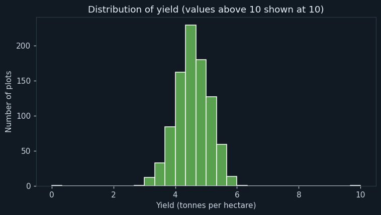
Each bar counts the plots whose yield falls in that range. Values above 10 are drawn at 10 so the one impossible value of 42 does not squash the chart.
Most plots yield between 3 and 6 t/ha, in a single hump — what a healthy yield distribution looks like. The thin bar at the far right is the impossible 42, drawn at 10. A histogram is the quickest way to spot such values before they mislead a model.
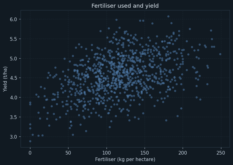
Each dot is a plot: fertiliser across, yield up.
Yield rises with fertiliser at first and then flattens: going from 0 to 100 kg/ha adds much more than going from 150 to 250. That curve is the most important thing in the dataset, for two reasons. It is the evidence that heavy fertiliser use is wasteful, and it tells us a straight-line model will struggle — which is why a Random Forest is tried as well.
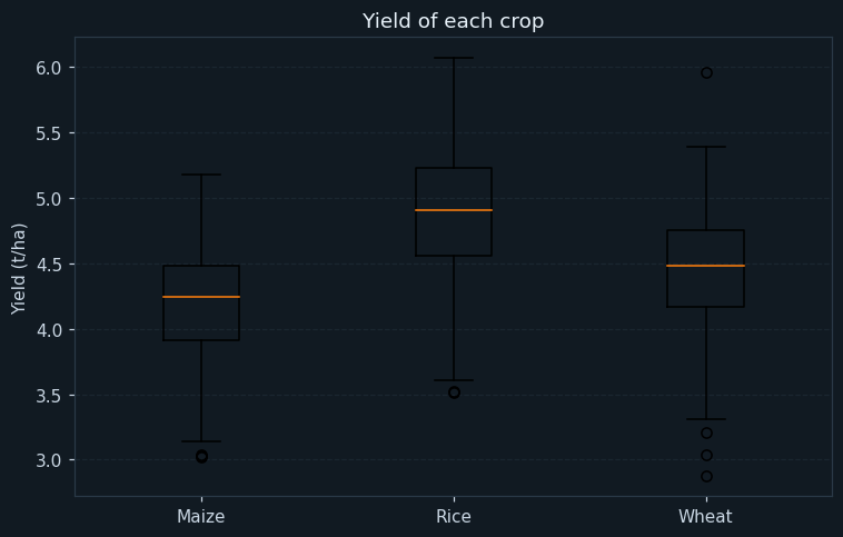
One box per crop. The line inside the box is the median, the box holds the middle half of the plots, and the whiskers reach the rest; dots beyond them are unusual plots.
Rice yields the most (median 4.91 t/ha), then wheat (4.48 t/ha) and maize (4.24 t/ha). The boxes overlap a good deal, so the crop alone cannot predict yield — but it shifts the whole range, which is why crop must be a feature.
7Step 6 — Data Preparation
drop_duplicates() removes exact repeats, which would otherwise count one plot twice and could appear in both the training and the testing data.
strip() and title() make them Rice, Wheat and Maize — otherwise the model would see six crops instead of three.
A yield of 42 t/ha (a decimal point lost) and one of −1 cannot be real. Rows with yield of 0 or less, or above 15 t/ha, are removed. Guessing the intended value would be inventing data.
Removing these rows would waste good yield records. They are filled with the median rainfall of the same crop, because rice plots receive far more rain than wheat plots — one overall median would be wrong for both. The median is used rather than the mean because it is not pulled by extreme values.
Feature engineering
Machine learning models need numbers. irrigated becomes 1 for Yes and 0 for No. crop is one-hot encoded with get_dummies(): three new columns, crop_Rice, crop_Wheat and crop_Maize, each 1 or 0. One-hot encoding is used instead of numbering the crops 1, 2, 3 because a number would tell the model that maize is "more" than rice — which means nothing.
That gives nine features. The plot ID is not one of them: an ID carries no information about yield, and a model given it could only memorise.
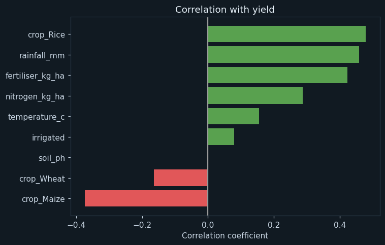
The Pearson correlation of each prepared feature with yield, from −1 to +1. Green bars move with yield, red bars against it.
Being a rice plot, rainfall and fertiliser have the strongest positive correlations; being a maize plot the strongest negative, because maize yields less per hectare in this region. Soil pH shows almost no correlation — but that does not mean it does not matter. pH hurts yield when it is too low or too high, so its effect is a curve that a correlation coefficient, which only measures straight-line relationships, cannot see. The Random Forest's feature importance (chart 8) tells a different story.
8Step 7 — Modelling
Every training plot comes with its harvested yield — the label — so this is supervised learning, and because the label is a number it is regression.
The data is split with train_test_split() into 718 plots for training and 180 for testing (80 : 20, as the handbook recommends for a dataset of this size), with a fixed random_state so the split is the same every run.
How the models work
Linear Regression fits one straight-line equation: yield = intercept + coefficient₁ × rainfall + coefficient₂ × temperature + … It learned an intercept of 3.013 and a fertiliser coefficient of 0.0049 t/ha per kg — on average each extra kilogram of fertiliser adds about 5 kg of grain per hectare. That average hides the curve in chart 2: the first kilograms add much more than that, the last ones much less.
The Random Forest builds 200 decision trees, each on a random sample of the training plots and features, and averages their predictions. Each tree asks questions such as "is fertiliser above 140?" and "is this a rice plot?", so together they can follow curves and interactions a single line cannot. min_samples_leaf=3 stops any tree from memorising single plots.
9Step 8 — Evaluation
On the 180 test plots, Linear Regression scored an RMSE of 0.38 t/ha and R² of 0.544; the Random Forest an RMSE of 0.357 t/ha and R² of 0.597. The handbook's three regression metrics all agree: MAE is the average size of an error, MSE squares errors so big ones count more, and RMSE brings that back to tonnes per hectare.
A single split can mislead, so 5-fold cross validation was run as well. The mean RMSE across folds was 0.368 for Linear Regression and 0.358 for the Random Forest — the same ranking, with every row of data used for testing once.
The gap is real but small. An R² near 0.6 means the models explain about 60% of the variation in yield; the rest comes from things the data does not record — pests, sowing dates, seed variety. A capstone report should say so plainly rather than chasing a higher number: no model can predict what it was never told.
The Random Forest is chosen for deployment. Linear Regression remains useful alongside it, because its fertiliser coefficient is something a farmer can understand in one sentence.
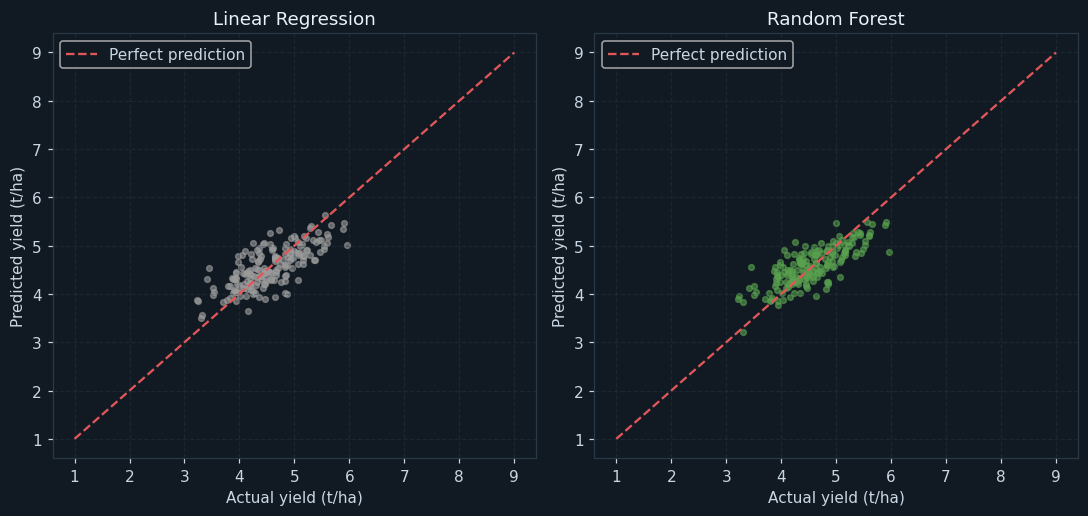
Each dot is a test plot: real yield across, prediction up, for Linear Regression (left) and the Random Forest (right). A perfect model puts every dot on the dashed line.
Both clouds follow the line. Look at the ends: Linear Regression's dots flatten towards the middle at both the low and the high end, because a straight line cannot bend to follow the fertiliser curve. The forest's dots stay closer to the line at the ends — the visual reason for its lower RMSE.
Neither cloud is tight. Some of the scatter cannot be removed: two plots with identical conditions still yield differently because of pests, sowing date and luck, none of which is in the data.
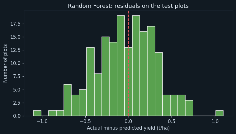
A residual is actual minus predicted yield for one test plot. Bars left of the red line are plots the model over-predicted; bars right of it, plots it under-predicted.
The residuals form one hump centred on zero — the mean residual is -0.034 t/ha — so the model is not biased high or low. 83.3 % of test plots are predicted within half a tonne per hectare. A lopsided or two-humped residual chart would have meant the model was missing something systematic.
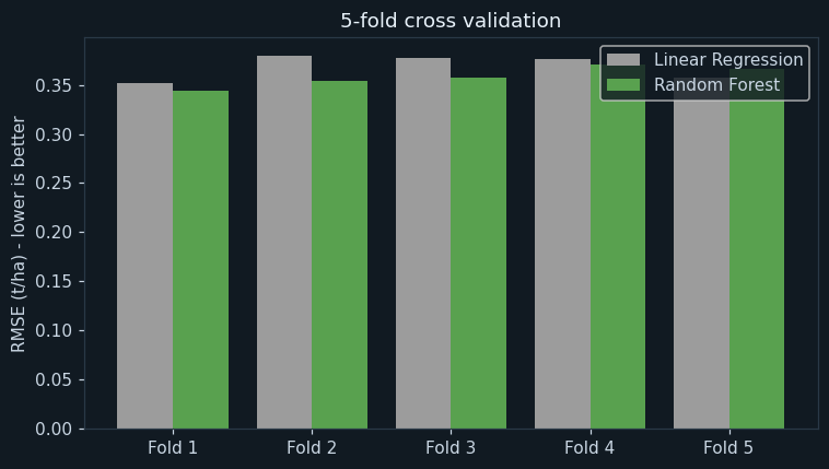
The RMSE of each model in each of the five folds. Each fold is a different fifth of the data, held out once.
The Random Forest has the lower error in most folds, and both models are consistent from fold to fold. That consistency is the point of cross validation: one train-test split could have been lucky or unlucky, but five folds agreeing means the comparison can be trusted.
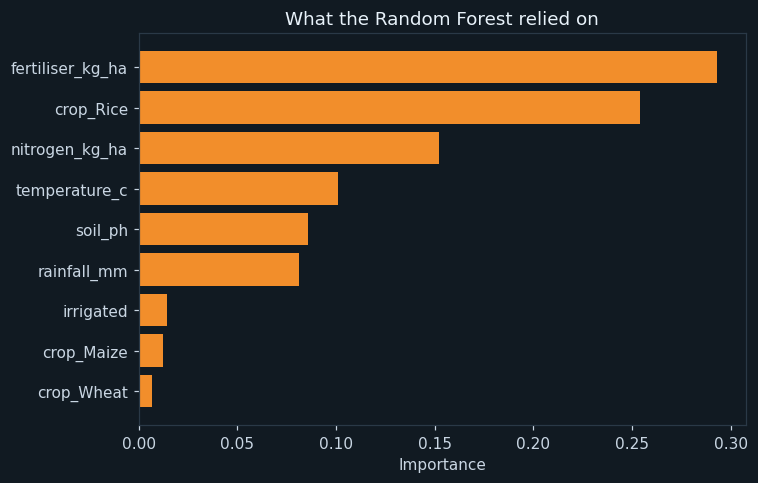
How much each feature contributed to the forest's decisions, adding up to 1.
Fertiliser and the crop matter most, then nitrogen, temperature and soil pH. Soil pH ranks well here although its correlation was zero — the forest can use its curved effect. Comparing charts 4 and 8 is a good viva answer: correlation and importance answer different questions.
10Step 9 — Deployment
The trained forest is saved with joblib.dump() to yield_model.pkl and loaded back with joblib.load(). An app or website — the curriculum's "website containing an ML model" activity — would load that file and predict without training again.
The program then predicts three new plots: a rain-fed rice plot after a good monsoon, an irrigated wheat plot, and a rain-fed maize plot with little fertiliser. In use, a farmer or extension worker would enter the plot's details mid-season and get a yield estimate with the typical error beside it: about ± 0.357 t/ha.
11Step 10 — Feedback
The last step closes the loop. After the next harvest, the real yields come back, and the model's predictions for that season can be checked against them. next_season.csv plays that role — and it is a drought year, with average rainfall falling from 837 mm to 558 mm.
The model's RMSE was 0.357 t/ha on last season's test data and 0.4 t/ha on the drought season. The program applies a simple rule: retrain if the error grows by more than 20%. Here it grew by about 12%, so the model stays in use — but the drift is real, and in a monitoring dashboard it would be the first warning sign.
Feedback from people matters as much as feedback from numbers. Farmers might report that predictions are too high on sandy soils, or for a new seed variety; each of those becomes a new feature or new training data, and the methodology loops back to Data Requirements.
12Ethical considerations
If most training plots come from larger, better-recorded farms, the model will be least accurate for the smallholders SDG 2 is about. The data must cover them deliberately.
A yield prediction must never be used to deny a farmer credit or insurance on its own — it has an error of about half a tonne per hectare. It supports decisions; it does not make them.
Plot-level records reveal a family's income. Data must be collected with consent, stored with plot IDs only, and shared only in aggregate.
The Random Forest is harder to explain than a line. Reporting feature importances and the Linear Regression coefficients alongside it keeps the reasoning visible to the people who rely on it.
13Source code
The whole program, laid out as the ten steps of the methodology. Every chart and number on this page came out of running it.
# ---------------------------------------------------------------------------
# crop_yield.py
#
# Capstone project: predicting the yield of a farm plot (tonnes per hectare)
# from its crop, weather, soil and the fertiliser used.
#
# CBSE Class XII, Artificial Intelligence (843), Part C - Capstone Project.
# SDG 2 (Zero Hunger) and SDG 12 (Responsible Consumption and Production).
#
# The program follows the 10 steps of the Data Science Methodology:
#   1 Business Understanding   2 Analytic Approach   3 Data Requirements
#   4 Data Collection          5 Data Understanding  6 Data Preparation
#   7 Modelling                8 Evaluation          9 Deployment
#   10 Feedback
#
# Two regression models are compared - Linear Regression, as in the
# handbook, and a Random Forest - with a train-test split and with 5-fold
# cross validation, using MAE, MSE, RMSE and R squared.
#
# Libraries: pandas, numpy, matplotlib, scikit-learn, joblib.
# ---------------------------------------------------------------------------

# %% Step 1 - Business Understanding
print("=" * 64)
print("HOW MUCH WILL THIS FIELD YIELD?")
print("=" * 64)
print("Problem : farmers and planners cannot tell before harvest how much")
print("          a plot will yield, so input use and storage are guesswork.")
print("Goal    : predict yield (t/ha) from crop, weather, soil and inputs.")
print()

# %% Step 2 - Analytic Approach
# The answer is a number (tonnes per hectare), so this is PREDICTIVE
# analytics using REGRESSION.
print("Analytic approach : predictive - regression (the target is a number)")
print()

# %% Step 3 - Data Requirements
import pandas as pd
import numpy as np
import matplotlib.pyplot as plt
from sklearn.model_selection import train_test_split, KFold, cross_val_score
from sklearn.linear_model import LinearRegression
from sklearn.ensemble import RandomForestRegressor
from sklearn.metrics import mean_absolute_error, mean_squared_error, r2_score
import joblib

pd.set_option("display.width", 130)
pd.set_option("display.max_columns", 20)

required = ["crop", "rainfall_mm", "temperature_c", "soil_ph", "nitrogen_kg_ha",
            "fertiliser_kg_ha", "irrigated", "yield_t_ha"]
print("Columns required :", required)

# %% Step 4 - Data Collection
data = pd.read_csv("crop_yield.csv")
print("Rows collected   :", len(data))
missing_columns = [c for c in required if c not in data.columns]
print("Required columns missing from the file :", missing_columns)
print()
print(data.head(8))
print()

# %% Step 5 - Data Understanding
print("--- Step 5: Data Understanding ---")
print("Missing values in each column:")
print(data.isnull().sum().to_string())
print()
print("Summary statistics:")
print(data.describe().round(2))
print()

# Chart 1: the distribution of yield.
plt.figure(figsize=(7, 4))
plt.hist(data["yield_t_ha"].clip(0, 10), bins=30, color="#59a14f", edgecolor="white")
plt.title("Distribution of yield (values above 10 shown at 10)")
plt.xlabel("Yield (tonnes per hectare)")
plt.ylabel("Number of plots")
plt.tight_layout()
plt.savefig("chart1_yield_distribution.png")
plt.close()

# Chart 2: fertiliser against yield.
ok = data[(data["yield_t_ha"] > 0) & (data["yield_t_ha"] < 15)]
plt.figure(figsize=(7, 5))
plt.scatter(ok["fertiliser_kg_ha"], ok["yield_t_ha"], s=12, alpha=0.5, color="#4e79a7")
plt.title("Fertiliser used and yield")
plt.xlabel("Fertiliser (kg per hectare)")
plt.ylabel("Yield (t/ha)")
plt.grid(True, linestyle="--", alpha=0.4)
plt.tight_layout()
plt.savefig("chart2_fertiliser_yield.png")
plt.close()

# Chart 3: yield of each crop, as box plots.
plt.figure(figsize=(7, 4.5))
crops_seen = sorted(ok["crop"].str.strip().str.title().unique())
plt.boxplot([ok[ok["crop"].str.strip().str.title() == c]["yield_t_ha"] for c in crops_seen], labels=crops_seen)
plt.title("Yield of each crop")
plt.ylabel("Yield (t/ha)")
plt.grid(True, axis="y", linestyle="--", alpha=0.4)
plt.tight_layout()
plt.savefig("chart3_yield_by_crop.png")
plt.close()
for c in crops_seen:
    part = ok[ok["crop"].str.strip().str.title() == c]["yield_t_ha"]
    print("Median yield of " + c.ljust(6), ":", round(part.median(), 2), "t/ha")
print()

# %% Step 6 - Data Preparation
print("--- Step 6: Data Preparation ---")
before = len(data)
data = data.drop_duplicates()
print("Duplicate rows removed          :", before - len(data))

data["crop"] = data["crop"].str.strip().str.title()
print("Crops after tidying the names   :", sorted(data["crop"].unique()))

impossible = ((data["yield_t_ha"] <= 0) | (data["yield_t_ha"] > 15)).sum()
data = data[(data["yield_t_ha"] > 0) & (data["yield_t_ha"] <= 15)]
print("Impossible yields removed       :", impossible)

# Missing rainfall is filled with the median rainfall of the same crop:
# rice fields get far more rain than wheat fields, so one overall median
# would be wrong for both.
blank_rain = data["rainfall_mm"].isnull().sum()
data["rainfall_mm"] = data.groupby("crop")["rainfall_mm"].transform(lambda s: s.fillna(s.median()))
print("Blank rainfall values filled    :", blank_rain, "(median of the same crop)")
print("Rows ready for modelling        :", len(data))

# Text columns become numbers. irrigated: Yes = 1, No = 0. crop: one
# column per crop (one-hot encoding), so no crop is treated as "bigger".
data["irrigated"] = (data["irrigated"] == "Yes").astype(int)
data = pd.get_dummies(data, columns=["crop"], dtype=int)
features = ["rainfall_mm", "temperature_c", "soil_ph", "nitrogen_kg_ha", "fertiliser_kg_ha",
            "irrigated", "crop_Maize", "crop_Rice", "crop_Wheat"]
print("Features used                   :", len(features))
print()

# Chart 4: correlation of every feature with yield.
corr = data[features + ["yield_t_ha"]].corr()["yield_t_ha"].drop("yield_t_ha").sort_values()
print("Correlation of each feature with yield:")
print(corr.round(2).to_string())
print()
plt.figure(figsize=(7, 4.5))
colours = ["#e15759" if v < 0 else "#59a14f" for v in corr.values]
plt.barh(corr.index, corr.values, color=colours)
plt.axvline(0, color="#999999")
plt.title("Correlation with yield")
plt.xlabel("Correlation coefficient")
plt.tight_layout()
plt.savefig("chart4_correlation.png")
plt.close()

# %% Step 7 - Modelling
print("--- Step 7: Modelling ---")
X = data[features]
y = data["yield_t_ha"]
X_train, X_test, y_train, y_test = train_test_split(X, y, test_size=0.2, shuffle=True, random_state=7)
print("Training rows :", len(X_train))
print("Testing rows  :", len(X_test))

linear = LinearRegression()
linear.fit(X_train, y_train)
forest = RandomForestRegressor(n_estimators=200, min_samples_leaf=3, random_state=0)
forest.fit(X_train, y_train)

print("Linear Regression - intercept :", round(linear.intercept_, 3))
print("Linear Regression - fertiliser coefficient :",
      round(linear.coef_[features.index("fertiliser_kg_ha")], 4), "t/ha per kg")
print()

# %% Step 8 - Evaluation
print("--- Step 8: Evaluation ---")
results = []
for name, model in [["Linear Regression", linear], ["Random Forest", forest]]:
    pred = model.predict(X_test)
    mae = mean_absolute_error(y_test, pred)
    mse = mean_squared_error(y_test, pred)
    rmse = np.sqrt(mse)
    r2 = r2_score(y_test, pred)
    results.append([name, mae, mse, rmse, r2])
    print(name)
    print("  " + name + " MAE  :", round(mae, 3), "t/ha")
    print("  " + name + " MSE  :", round(mse, 3))
    print("  " + name + " RMSE :", round(rmse, 3), "t/ha")
    print("  " + name + " R2   :", round(r2, 3))
print()

# 5-fold cross validation: every row is in the test fold exactly once.
folds = KFold(n_splits=5, shuffle=True, random_state=1)
cv_lin = np.sqrt(-cross_val_score(LinearRegression(), X, y, cv=folds, scoring="neg_mean_squared_error"))
cv_rf = np.sqrt(-cross_val_score(RandomForestRegressor(n_estimators=200, min_samples_leaf=3, random_state=0),
                                 X, y, cv=folds, scoring="neg_mean_squared_error"))
print("RMSE in each of the 5 folds (t/ha):")
print("  Fold  Linear  Forest")
for k in range(5):
    print("  ", k + 1, "  ", round(cv_lin[k], 3), " ", round(cv_rf[k], 3))
print("Mean cross-validated RMSE, Linear Regression :", round(cv_lin.mean(), 3))
print("Mean cross-validated RMSE, Random Forest     :", round(cv_rf.mean(), 3))
print()

best_pred = forest.predict(X_test)

# Chart 5: predicted against actual, for both models side by side.
lin_pred = linear.predict(X_test)
plt.figure(figsize=(10, 4.8))
for k in range(2):
    plt.subplot(1, 2, k + 1)
    pred = [lin_pred, best_pred][k]
    plt.scatter(y_test, pred, s=14, alpha=0.6, color=["#9c9c9c", "#59a14f"][k])
    plt.plot([1, 9], [1, 9], color="#e15759", linestyle="--", label="Perfect prediction")
    plt.title(["Linear Regression", "Random Forest"][k])
    plt.xlabel("Actual yield (t/ha)")
    plt.ylabel("Predicted yield (t/ha)")
    plt.legend()
    plt.grid(True, linestyle="--", alpha=0.4)
plt.tight_layout()
plt.savefig("chart5_predicted_actual.png")
plt.close()

# Chart 6: the residuals (actual minus predicted) of the forest.
residuals = y_test - best_pred
print("Mean residual (Random Forest)        :", round(residuals.mean(), 3), "t/ha")
print("Residuals within +/- 0.5 t/ha        :", round((residuals.abs() <= 0.5).mean() * 100, 1), "%")
plt.figure(figsize=(7, 4))
plt.hist(residuals, bins=25, color="#59a14f", edgecolor="white")
plt.axvline(0, color="#e15759", linestyle="--")
plt.title("Random Forest: residuals on the test plots")
plt.xlabel("Actual minus predicted yield (t/ha)")
plt.ylabel("Number of plots")
plt.tight_layout()
plt.savefig("chart6_residuals.png")
plt.close()

# Chart 7: RMSE in each fold for both models.
x = np.arange(5)
plt.figure(figsize=(7, 4))
plt.bar(x - 0.2, cv_lin, width=0.4, label="Linear Regression", color="#9c9c9c")
plt.bar(x + 0.2, cv_rf, width=0.4, label="Random Forest", color="#59a14f")
plt.xticks(x, ["Fold 1", "Fold 2", "Fold 3", "Fold 4", "Fold 5"])
plt.ylabel("RMSE (t/ha) - lower is better")
plt.title("5-fold cross validation")
plt.legend()
plt.tight_layout()
plt.savefig("chart7_kfold.png")
plt.close()

# Chart 8: which features the forest relied on.
importance = pd.Series(forest.feature_importances_, index=features).sort_values()
print("Feature importance (Random Forest):")
print(importance.round(3).to_string())
print()
plt.figure(figsize=(7, 4.5))
plt.barh(importance.index, importance.values, color="#f28e2b")
plt.title("What the Random Forest relied on")
plt.xlabel("Importance")
plt.tight_layout()
plt.savefig("chart8_importance.png")
plt.close()

# %% Step 9 - Deployment
print("--- Step 9: Deployment ---")
# The trained model is saved to a file, so an app or website can load it
# and predict without training again.
joblib.dump(forest, "yield_model.pkl")
loaded = joblib.load("yield_model.pkl")
print("Model saved to yield_model.pkl and loaded back")

new_plots = pd.DataFrame({
    "rainfall_mm": [1180, 560, 640], "temperature_c": [26.5, 18.5, 27.0], "soil_ph": [6.7, 7.1, 7.9],
    "nitrogen_kg_ha": [85, 90, 60], "fertiliser_kg_ha": [130, 150, 40], "irrigated": [0, 1, 0],
    "crop_Maize": [0, 0, 1], "crop_Rice": [1, 0, 0], "crop_Wheat": [0, 1, 0],
})
names = ["Rice, rain-fed, good rain", "Wheat, irrigated", "Maize, rain-fed, little fertiliser"]
predicted = loaded.predict(new_plots)
for i in range(len(names)):
    print(names[i].ljust(36), "->", round(predicted[i], 2), "t/ha")
print()

# %% Step 10 - Feedback
print("--- Step 10: Feedback ---")
# After the next season's harvest, the real yields come back. Comparing
# them with what the model predicted shows whether it still works.
nxt = pd.read_csv("next_season.csv")
nxt["irrigated"] = (nxt["irrigated"] == "Yes").astype(int)
nxt = pd.get_dummies(nxt, columns=["crop"], dtype=int)
next_pred = loaded.predict(nxt[features])
next_rmse = np.sqrt(mean_squared_error(nxt["yield_t_ha"], next_pred))
print("Plots in the next season's feedback :", len(nxt))
print("RMSE on last season's test data     :", round(results[1][3], 3), "t/ha")
print("RMSE on the next season             :", round(next_rmse, 3), "t/ha")
print("Average rainfall, training season   :", round(data["rainfall_mm"].mean()), "mm")
print("Average rainfall, next season       :", round(nxt["rainfall_mm"].mean()), "mm")
if next_rmse > 1.2 * results[1][3]:
    print("Feedback: error has grown by more than 20% - retrain with the new season's data.")
else:
    print("Feedback: error is within 20% of last season - the model can stay in use.")
The library calls it is built from
| Call | Step | What it does |
|---|---|---|
pd.read_csv() | Step 4 | Reads the dataset into a DataFrame |
isnull().sum() / describe() | Step 5 | Counts missing values; summary statistics |
drop_duplicates() | Step 6 | Removes repeated rows |
groupby().transform(... fillna(median)) | Step 6 | Fills blank rainfall with the median of the same crop |
pd.get_dummies() | Step 6 | One-hot encodes the crop column |
DataFrame.corr() | Step 6 | Pearson correlation of each feature with yield |
train_test_split(test_size=0.2) | Step 7 | Splits into 80% training and 20% testing data |
LinearRegression().fit() | Step 7 | Trains the linear model |
RandomForestRegressor().fit() | Step 7 | Trains the forest of 200 trees |
mean_absolute_error / mean_squared_error / r2_score | Step 8 | The regression metrics |
KFold + cross_val_score() | Step 8 | 5-fold cross validation |
feature_importances_ | Step 8 | What the forest relied on |
joblib.dump() / joblib.load() | Step 9 | Saves and reloads the trained model |
14Output of a real run
================================================================
HOW MUCH WILL THIS FIELD YIELD?
================================================================
Problem : farmers and planners cannot tell before harvest how much
          a plot will yield, so input use and storage are guesswork.
Goal    : predict yield (t/ha) from crop, weather, soil and inputs.

Analytic approach : predictive - regression (the target is a number)

Columns required : ['crop', 'rainfall_mm', 'temperature_c', 'soil_ph', 'nitrogen_kg_ha', 'fertiliser_kg_ha', 'irrigated', 'yield_t_ha']
Rows collected   : 904
Required columns missing from the file : []

  plot_id   crop  rainfall_mm  temperature_c  soil_ph  nitrogen_kg_ha  fertiliser_kg_ha irrigated  yield_t_ha
0  P10001  Maize        759.0           26.3      6.1            84.0             121.0        No        4.79
1  P10002   Rice       1448.0           23.6      6.4            72.0              99.0        No        4.49
2  P10003   Rice       1278.0           28.6      5.9            75.0              53.0       Yes        4.24
3  P10004   Rice       1139.0           27.3      7.6            72.0             122.0       Yes        5.34
4  P10005   Rice       1245.0           26.3      6.3           127.0             116.0       Yes        5.39
5  P10006  Wheat        797.0           23.1      6.5            54.0              95.0        No        4.83
6  P10006  Wheat        797.0           23.1      6.5            54.0              95.0        No        4.83
7  P10007  Maize        624.0           28.5      6.8            78.0              71.0       Yes        3.47

--- Step 5: Data Understanding ---
Missing values in each column:
plot_id              0
crop                 0
rainfall_mm         18
temperature_c        0
soil_ph              0
nitrogen_kg_ha       0
fertiliser_kg_ha     0
irrigated            0
yield_t_ha           0

Summary statistics:
       rainfall_mm  temperature_c  soil_ph  nitrogen_kg_ha  fertiliser_kg_ha  yield_t_ha
count       886.00         904.00   904.00          904.00            904.00      904.00
mean        837.04          24.00     6.80           79.28            117.68        4.60
std         318.87           4.58     0.59           24.02             46.41        1.37
min         160.00           9.20     4.80           10.00              0.00       -1.00
25%         593.00          20.08     6.40           62.00             88.00        4.22
50%         772.00          25.15     6.80           80.00            117.00        4.57
75%        1073.00          27.70     7.20           96.00            147.00        4.94
max        1824.00          33.20     8.50          140.00            249.00       42.00

Median yield of Maize  : 4.24 t/ha
Median yield of Rice   : 4.91 t/ha
Median yield of Wheat  : 4.48 t/ha

--- Step 6: Data Preparation ---
Duplicate rows removed          : 4
Crops after tidying the names   : ['Maize', 'Rice', 'Wheat']
Impossible yields removed       : 2
Blank rainfall values filled    : 18 (median of the same crop)
Rows ready for modelling        : 898
Features used                   : 9

Correlation of each feature with yield:
crop_Maize         -0.37
crop_Wheat         -0.16
soil_ph            -0.00
irrigated           0.08
temperature_c       0.15
nitrogen_kg_ha      0.29
fertiliser_kg_ha    0.42
rainfall_mm         0.46
crop_Rice           0.48

--- Step 7: Modelling ---
Training rows : 718
Testing rows  : 180
Linear Regression - intercept : 3.013
Linear Regression - fertiliser coefficient : 0.0049 t/ha per kg

--- Step 8: Evaluation ---
Linear Regression
  Linear Regression MAE  : 0.302 t/ha
  Linear Regression MSE  : 0.144
  Linear Regression RMSE : 0.38 t/ha
  Linear Regression R2   : 0.544
Random Forest
  Random Forest MAE  : 0.286 t/ha
  Random Forest MSE  : 0.128
  Random Forest RMSE : 0.357 t/ha
  Random Forest R2   : 0.597

RMSE in each of the 5 folds (t/ha):
  Fold  Linear  Forest
   1    0.352   0.344
   2    0.379   0.354
   3    0.378   0.357
   4    0.376   0.371
   5    0.358   0.366
Mean cross-validated RMSE, Linear Regression : 0.368
Mean cross-validated RMSE, Random Forest     : 0.358

Mean residual (Random Forest)        : -0.034 t/ha
Residuals within +/- 0.5 t/ha        : 83.3 %
Feature importance (Random Forest):
crop_Wheat          0.007
crop_Maize          0.012
irrigated           0.014
rainfall_mm         0.081
soil_ph             0.086
temperature_c       0.101
nitrogen_kg_ha      0.152
crop_Rice           0.254
fertiliser_kg_ha    0.293

--- Step 9: Deployment ---
Model saved to yield_model.pkl and loaded back
Rice, rain-fed, good rain            -> 5.19 t/ha
Wheat, irrigated                     -> 4.74 t/ha
Maize, rain-fed, little fertiliser   -> 3.76 t/ha

--- Step 10: Feedback ---
Plots in the next season's feedback : 120
RMSE on last season's test data     : 0.357 t/ha
RMSE on the next season             : 0.4 t/ha
Average rainfall, training season   : 837 mm
Average rainfall, next season       : 558 mm
Feedback: error is within 20% of last season - the model can stay in use.15The same project in Orange
The curriculum allows the capstone in Orange, and Unit 4 teaches it. The same workflow, widget by widget: The tool is Orange Data Mining.
| Widget | What it does |
|---|---|
| File | Load crop_yield.csv; set yield_t_ha as the target and plot_id as a meta attribute. |
| Feature Statistics / Distributions | Spot the blank rainfall and the impossible yields (Step 5). |
| Select Rows + Impute + Preprocess | Remove impossible yields; impute missing rainfall; Orange's learners encode categories automatically (Step 6). |
| Scatter Plot | Plot fertiliser against yield, as in chart 2. |
| Linear Regression and Random Forest | The two learners (Step 7). |
| Test and Score | Choose Cross validation with 5 folds; read MSE, RMSE, MAE and R² for both models (Step 8). |
| Predictions | Feed in new plots to predict their yield (Step 9). |
16Testing
Every case was run: each gives the whole program a small input of its own.
| Test case | Expected | Actual | Result |
|---|---|---|---|
| The full dataset | Rows collected : 904 | Rows collected : 904 | Pass |
| Four duplicated rows are removed | Duplicate rows removed : 4 | Duplicate rows removed : 4 | Pass |
| "rice", " WHEAT" and "maize " join their crops | Crops after tidying the names : ['Maize', 'Rice', 'Wheat'] | Crops after tidying the names : ['Maize', 'Rice', 'Wheat'] | Pass |
| A yield of 42 t/ha and one of -1 are impossible | Impossible yields removed : 2 | Impossible yields removed : 2 | Pass |
| Blank rainfall is filled, not dropped | Blank rainfall values filled : 18 (median of the same crop) | Blank rainfall values filled : 18 (median of the same crop) | Pass |
| The forest beats the straight line in cross validation | Mean cross-validated RMSE, Random Forest : 0.358 | Mean cross-validated RMSE, Random Forest : 0.358 | Pass |
| Yield that is an exact straight-line rule: Linear Regression finds it (R2 = 1) | Linear Regression R2 : 1.0 | Linear Regression R2 : 1.0 | Pass |
| Boundary: 15.0 t/ha is kept, 15.01 is removed | Impossible yields removed : 1 | Impossible yields removed : 1 | Pass |
| The data file is missing | FileNotFoundError: [Errno 2] No such file or directory: 'crop_yield.csv' | FileNotFoundError: [Errno 2] No such file or directory: 'crop_yield.csv' | Pass |
17Team roles and timeline
A capstone is done by a group of 3 to 5. A suggested split of the work, and a timeline across the year:
| Role | Responsible for |
|---|---|
| Project lead | Business understanding, the 5W1H canvas, meeting the farmers and officers, the final presentation |
| Data lead | Data requirements and collection: the survey, IMD and Soil Health Card data, permissions |
| Analyst | Data understanding and preparation: cleaning, filling missing values, encoding, charts |
| Modeller | Training and comparing the models, cross validation, choosing the final model |
| Documentation and video | The project documentation, the 3-minute video script and editing |
| When | Methodology steps | Deliverable |
|---|---|---|
| April – May | 1 Business Understanding, 2 Analytic Approach | Problem statement and 5W1H canvas approved by the teacher |
| June – July | 3 Data Requirements, 4 Data Collection | Survey done; secondary data downloaded and credited |
| August | 5 Data Understanding, 6 Data Preparation | Clean dataset and exploratory charts |
| September – October | 7 Modelling, 8 Evaluation | Models compared with K-fold; final model chosen |
| November | 9 Deployment, 10 Feedback | Saved model, predictions, feedback plan |
| December – January | Documentation and video | Report, 3-minute video, viva preparation |
18Results, limits and what next
- Both models predict yield to within about 0.36–0.38 t/ha on unseen plots; the Random Forest is slightly but consistently better.
- Cross validation confirms the ranking: mean RMSE 0.358 for the forest against 0.368 for the line.
- Fertiliser has diminishing returns — the first 100 kg/ha add far more than the next 100.
- Soil pH matters although its correlation with yield is zero, because its effect is a curve.
- In a drought season the model's error grew by about 12%: still usable, but drifting.
Limitations
- Sample data from one region; real yields vary far more between districts
- No information on pests, sowing date, seed variety or soil type
- About 40% of the variation in yield is not explained by the features available
- The model has seen only one season; one drought year in the feedback is not enough to judge it fully
Future scope
- Add sowing date, seed variety and a pest-incidence score as features
- Collect several seasons and test on a whole season held out (time-based validation)
- Recommend the fertiliser dose with the best yield per rupee — a step into prescriptive analytics
- Build a simple web form around yield_model.pkl, as in the curriculum's website activity
What the team had to learn
- Regression metrics: MAE, MSE, RMSE and R², and when each is useful
- K-fold cross validation with scikit-learn, and why it is more reliable than one split
- One-hot encoding categorical features
- Why correlation can miss a curved relationship that a tree-based model finds
19Conclusion
The capstone followed all ten steps of the Data Science Methodology to answer one question: can a plot's yield be predicted before harvest? It can — to within about a third of a tonne per hectare, with a Random Forest that cross validation confirms is slightly better than Linear Regression.
The most useful result for SDG 2 and 12 is not the prediction itself but what the data showed along the way: fertiliser's effect flattens out, so the heaviest doses add little but cost. That is a finding a farmer can act on this season.
The feedback step showed the methodology's last lesson. A model is not finished when it is deployed; it must be checked against each new season, and a drought year is exactly when it starts to drift.
20The 3-minute video script
Part C asks for a video of exactly three minutes with six parts. A script, timed to the second:
| Time | Part | What to say and show |
|---|---|---|
| 0:00 – 0:25 | a. Problem statement | Show a field and a mandi. "Before harvest, nobody knows how much a field will yield — so fertiliser, storage and procurement are guesswork. Our problem statement: …" |
| 0:25 – 0:45 | b. SDG alignment | Show the SDG 2 and SDG 12 icons. "More food from the same land, and less fertiliser wasted." |
| 0:45 – 1:20 | c. AI concepts and algorithms | "This is predictive analytics using supervised regression. We compared Linear Regression and a Random Forest, using a train-test split and 5-fold cross validation, judged by MAE, MSE and RMSE." Show the methodology wheel. |
| 1:20 – 2:20 | d. How it works | Screen-record the notebook: the cleaning counts, chart 2 (fertiliser curve), the K-fold chart, then the three new plots being predicted. End on the feedback lines for the drought season. |
| 2:20 – 2:45 | e. Conclusion | "Our model predicts yield within about a third of a tonne. Fertiliser beyond about 150 kg/ha adds very little — and the model must be checked every season." |
| 2:45 – 3:00 | f. Acknowledgement | "We thank our AI teacher, [name], and the farmers who shared their records." Show the team. |
21Questions for the viva
▸Which type of analytics is your project, and why?
Predictive analytics, because it forecasts a future outcome — the yield — from past data. It uses regression because the target is a number.
▸Why did you fill missing rainfall with the median of the same crop?
Rice and wheat plots receive very different rainfall, so one overall value would be wrong for both. The median is used because extreme values do not pull it.
▸What is the difference between MSE and RMSE?
MSE is the average of the squared errors. RMSE is its square root, so it is in the same units as yield — tonnes per hectare — and easier to interpret.
▸Why did you use K-fold cross validation as well as a train-test split?
One split can be lucky or unlucky. K-fold uses every row as test data once, giving five measurements, so the comparison between the models is more reliable.
▸Soil pH has zero correlation with yield. Does it matter?
Yes. Its effect is a curve — yield falls when pH is too low or too high — and correlation only measures straight-line relationships. The Random Forest's importance shows it matters.
▸What does one-hot encoding do?
It turns a text category into several 0/1 columns, one per category, so the model does not treat the categories as numbers with an order.
▸What did the Feedback step tell you?
In a drought season the error grew by about 12%, under our 20% retraining rule. The model can stay in use but should be watched.
▸Which SDGs is your project aligned to?
SDG 2, Zero Hunger, and SDG 12, Responsible Consumption and Production.
22References
- Directorate of Economics and Statistics, Ministry of Agriculture & Farmers Welfare — district-wise crop production data — https://desagri.gov.in/
- India Meteorological Department — district rainfall — https://mausam.imd.gov.in/
- Soil Health Card scheme — https://soilhealth.dac.gov.in/
- Open Government Data Platform India — https://data.gov.in/
- CBSE, Artificial Intelligence (Subject Code 843), Class XII curriculum, 2026-27 — Part C
- CBSE, Artificial Intelligence Student Handbook, Class XII — Unit 2, Data Science Methodology
- Rollins, J. B. (2015). Foundational Methodology for Data Science. IBM Analytics.
- scikit-learn — https://scikit-learn.org/stable/; pandas, NumPy and Matplotlib documentation
- LambdaLab — https://www.lambdalab.in