The Mid-Day Meal Story
The curriculum's own data-storytelling capstone: thirty-five years of enrolment, attendance and dropout, told on Freytag's pyramid — with the diagnostic analysis to back the story, and the honesty to say what the data cannot prove.
1Introduction
The Mid-Day Meal Scheme began in 1995, and from 2001 every government primary school had to serve a cooked meal. It is one of the largest school feeding programmes in the world. But a programme like this has to keep earning its budget, and the question asked of it every year is simple: has it worked?
The numbers to answer that question exist — enrolment, attendance and dropout, year after year. But a spreadsheet of thirty-five years is not an answer. Officials, parents and journalists need a story they can follow: what things were like, what changed, and what it led to.
The CBSE curriculum sets exactly this as its sample data-storytelling problem: use enrolment, attendance and dropout data to tell a compelling, honest story about the scheme's impact, including external factors that may have shaped the trends. This capstone does that, following the Data Science Methodology — and adds the diagnostic analysis that tells the storyteller which claims the data supports.
Quality Education
Zero Hunger
The Mid-Day Meal Scheme — PM POSHAN since 2021 — sits exactly where SDG 2 and SDG 4 meet: a hot meal at school feeds a hungry child and gives the family a reason to keep that child in class. Showing clearly what happened to enrolment and dropout as the scheme grew is how a programme's value is argued for, defended and improved.
2Step 1 — Business Understanding
What is the problem that you are trying to solve? The handbook uses the 5W1H Problem Canvas for this step.
- • State education department officials
- • School management committees and parents
- • Journalists and the public
- • Thirty-five years of school data that nobody reads as a whole
- • The scheme's impact is asserted or doubted without evidence
- • Government primary schools in one state
- • 1990 to 2024 — before the scheme, through its growth, and after COVID-19
- • A clear, honest story helps defend and improve a programme that feeds millions of children
- • Getting the story wrong — claiming too much — damages trust in the data
- • Describe each period, test whether the trend changed when cooked meals began, and tell the result on Freytag's pyramid
Problem statement
Who would use it: Education department officials reviewing the scheme, school management committees, journalists and policy students — and anyone who has to explain the scheme's effect to a non-specialist audience.
Talking to the stakeholders
The handbook pairs the 5W1H canvas with Design Thinking, which begins by empathising with the people who have the problem. The questions asked, and what each answer changed:
| Question asked | What we learned, and what it changed |
|---|---|
| To a headteacher: what changed in your school when cooked meals began? | Attendance in the afternoon rose — children stayed after lunch. This made attendance, not just enrolment, a measure to include. |
| To a headteacher: what else changed at about the same time? | New classrooms under Sarva Shiksha Abhiyan, and later the Right to Education Act. This set up the external-factors part of the story: meals were not the only change. |
| To parents: why do children leave primary school? | Work at home or in the fields, distance, and for girls, safety and chores. The data needed the girls' share of enrolment to see whether the scheme reached girls. |
| To a block education officer: which figures are reported every year? | Enrolment, average attendance and dropout, plus the share of schools serving meals. That fixed the data requirements. |
| To a block education officer: is any year's data unreliable? | 1998's attendance records were lost in a flood, and 2020 had no attendance because schools were closed. Both became data preparation decisions, made differently. |
| To a journalist: what makes a data story believable? | One clear claim, a chart that shows it, and an honest statement of what it does not prove. That shaped the ethics section and the headline chart. |
How it is handled today
Accurate tables, published every year. They describe one year at a time and rarely show the thirty-year picture.
Detailed studies exist, but they are long and technical. A school committee or a parent will not read them.
Clear and memorable, but often claim the scheme alone caused every improvement — a claim the data cannot fully support, which undermines trust when it is noticed.
Objectives
- To frame the scheme's impact as a question that data can answer, using the 5W1H canvas
- To collect and understand a 35-year series of enrolment, attendance, dropout and meal coverage
- To prepare the data carefully — treating a lost record and a closure year differently
- To compare the periods before the scheme, with dry rations, and with cooked meals
- To test, with two regression models and leave-one-out cross validation, whether the dropout trend really changed when cooked meals began
- To tell the result as a data story on Freytag's pyramid, with a headline chart
- To state clearly what the story does not prove, and how new data will test it
3Step 2 — Analytic Approach
The first questions are descriptive — what happened to enrolment, attendance and dropout, and how did each period compare? The handbook's descriptive analytics summarises historical data with means and trends.
The central question is diagnostic: did the dropout trend change when cooked meals began, and by how much? Diagnostic analytics looks for the reasons behind an outcome, using correlation and comparing patterns before and after an event. Regression is used here not to predict the future but to measure how steeply dropout fell in each period.
Prediction is deliberately not the goal. A data story about a programme's past must explain, not forecast.
| Candidate | Why it was considered |
|---|---|
| Period averages (descriptive) | The simplest honest comparison: average dropout, attendance and enrolment before the scheme, with dry rations, and with cooked meals. |
| Correlation (diagnostic) | How closely meal coverage moves with dropout and attendance across the years — strong correlation is evidence, not proof. |
| Linear Regression, one line (Model A) | Assumes dropout fell at one steady rate throughout — the 'nothing special happened' explanation. |
| Segmented Linear Regression (Model B) | Lets the slope change in 2001 and 2012. If it fits clearly better, the trend really did change at those points. |
4Step 3 — Data Requirements
To compare before and after, the data must start well before 1995 and run long after 2001 — at least five years either side of each event. It must be structured, one row per year, with numbers for every measure.
Because the curriculum asks for external factors, the data requirements include dates of other events — the Right to Education Act, COVID-19 closures — even though they are not columns of the table: they are the context the story needs.
| Data needed | Type | Format | Source |
|---|---|---|---|
| Year | Numeric (integer) | 1990 – 2024 | — |
| Enrolment in primary schools | Numeric | Lakh children | UDISE+ / state education department |
| Girls' share of enrolment | Numeric | Percentage | UDISE+ |
| Average attendance | Numeric | Percentage | State education department |
| Dropout rate, primary | Numeric | Percentage | UDISE+ |
| Schools serving meals | Numeric | Percentage | PM POSHAN / Mid-Day Meal Scheme reports |
| Dates of external events | Text | Year and description | Government notifications, court records |
5Step 4 — Data Collection
In a real project almost all of this is secondary data — collected by the government and published. UDISE+ (Unified District Information System for Education Plus) publishes enrolment and dropout; the Ministry of Education publishes PM POSHAN coverage; older years come from the archived annual reports. Interviews with teachers and officials are primary data and add the human side of the story.
The sample file, school_data.csv, holds 36 rows covering 1990 to 2024 for one imaginary state, shaped around the scheme's real milestones: its launch on 15 August 1995 as the National Programme of Nutritional Support to Primary Education; the Supreme Court's order of 28 November 2001 that every government primary school serve a cooked meal; the Right to Education Act coming into force on 1 April 2010; the COVID-19 closures of 2020–21; and the renaming to PM POSHAN in 2021.
The milestones are real; the numbers are not. A capstone using this project must replace them with real figures for its own state, and credit the sources.
| Column | Type | What it holds | Role |
|---|---|---|---|
year | integer | The school year | time axis |
enrolment_lakh | decimal | Children enrolled in primary classes, in lakh | measure |
girls_share_pct | decimal | Girls as a percentage of enrolment | measure |
attendance_pct | decimal | Average daily attendance, % | measure |
dropout_pct | decimal | Primary-level dropout rate, % | target of the trend models |
meal_coverage_pct | integer | Schools serving a meal, % | measure |
period | text | Before the scheme / Dry rations / Cooked meals — made by the program | engineered |
years_since_2001, years_since_2012 | integer | Years after each break point, 0 before it — made by the program | engineered features |
school_data.csv — One row per year, 1990 to 2024, for one state's government primary schools. 36 rows, 1.1 KB. Download the file
The first ten rows of school_data.csv
| year | enrolment_lakh | girls_share_pct | attendance_pct | dropout_pct | meal_coverage_pct |
|---|---|---|---|---|---|
1990 | 40.8 | 43.4 | 60.1 | 38.5 | 0 |
1991 | 41.6 | 43.6 | 60.1 | 38.1 | 0 |
1992 | 42.5 | 43.9 | 61.8 | 36.8 | 0 |
1993 | 42.7 | 43.8 | 60.7 | 36.2 | 0 |
1994 | 42.8 | 43.8 | 61.5 | 36.0 | 0 |
1995 | 43.5 | 43.7 | 62.2 | 35.7 | 35 |
1996 | 44.8 | 44.3 | 63.1 | 34.7 | 38 |
1997 | 44.5 | 44.3 | 62.2 | 34.3 | 41 |
1998 | 45.4 | 44.5 | | 34.0 | 44 |
1999 | 46.2 | 44.6 | 62.6 | 32.7 | 47 |
6Step 5 — Data Understanding
Is the data collected representative of the problem to be solved?
The data must represent the problem: thirty-five consecutive years, all five measures, no gaps except where the officer warned there would be. The checks confirm two missing attendance values — 1998 and 2020 — and one duplicated year.
Chart 1 is the first look at the central measure. Dropout falls throughout, but not evenly: gently before 2001, steeply from 2001 to about 2012, then flat, with a bump in 2020–21. That shape, visible before any model is built, shapes everything that follows — including the decision in Step 6 to let the trend bend at 2001 and 2012.
Chart 2 shows enrolment rising steadily and the girls' share creeping up — so the story is not only about fewer children leaving, but more children, and more girls, arriving.
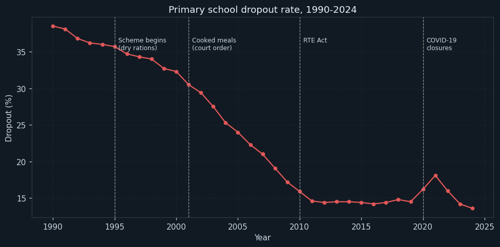
Dropout rate each year, with dashed lines at the scheme's launch, the cooked-meal order, the RTE Act and the COVID-19 closures.
The line falls the whole time, but at three different speeds — slowly before 2001, fast from 2001 to about 2012, barely at all after that — with a rise in 2020–21 when schools closed. A good data story follows the shape of its data, and this shape already suggests the story's structure.
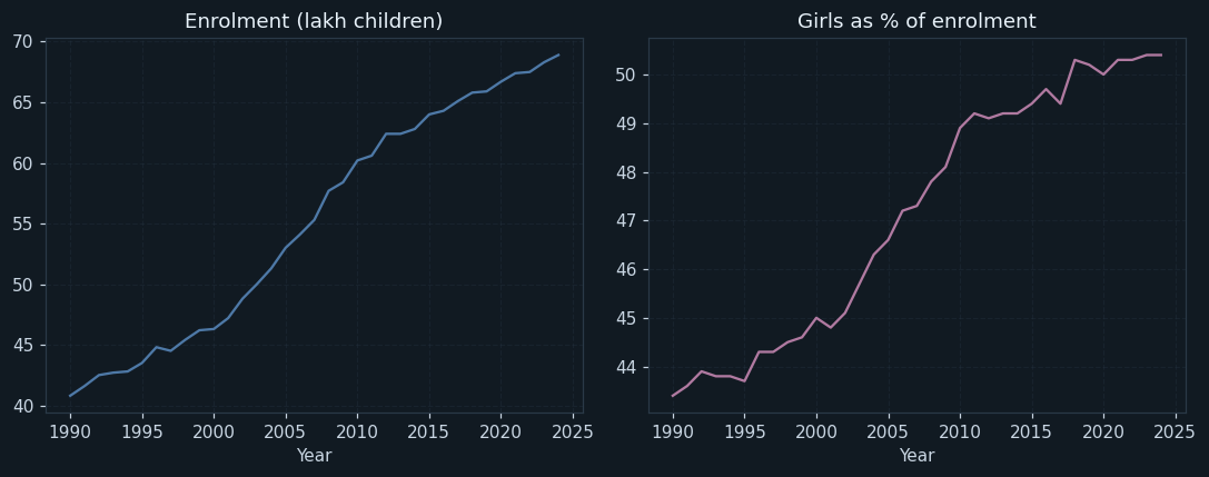
Left: children enrolled, in lakh. Right: girls as a percentage of enrolment.
Enrolment rises steadily and faster after 2001, and the girls' share climbs from about 43% to about 50%. The scheme's story is therefore also about access: more children came to school, and more of them were girls.
7Step 6 — Data Preparation
drop_duplicates() removes it. A repeated year would count twice in every period average and pull the trend line.
Filled by linear interpolation — the value halfway along the line from 1997 to 1999, giving 62.4%. Interpolation suits a smooth yearly series where the neighbours are known; it is stated in the report so a reader knows that value is an estimate.
Left missing on purpose. There was no attendance to record; filling it with an average would hide the single most important fact about that year. Treating two missing values differently, for stated reasons, is the data preparation lesson of this project.
Kept in the data and the story, but left out of the trend models, which use 1990–2019. A pandemic is an outside shock; fitting it would distort the measured effect of meals.
Feature engineering
A period column labels each year Before the scheme (to 1994), Dry rations (1995–2000) or Cooked meals (2001 onward), so the program can compare the three with groupby().
For the trend model, two features — years_since_2001 and years_since_2012 — are 0 before each break and count the years after it. Added to an ordinary regression on year, they let the fitted line change its slope at exactly those points: this is segmented regression, built from Linear Regression and feature engineering alone. The break points were not invented — chart 1 shows the fall steepening at 2001 and flattening at 2012.
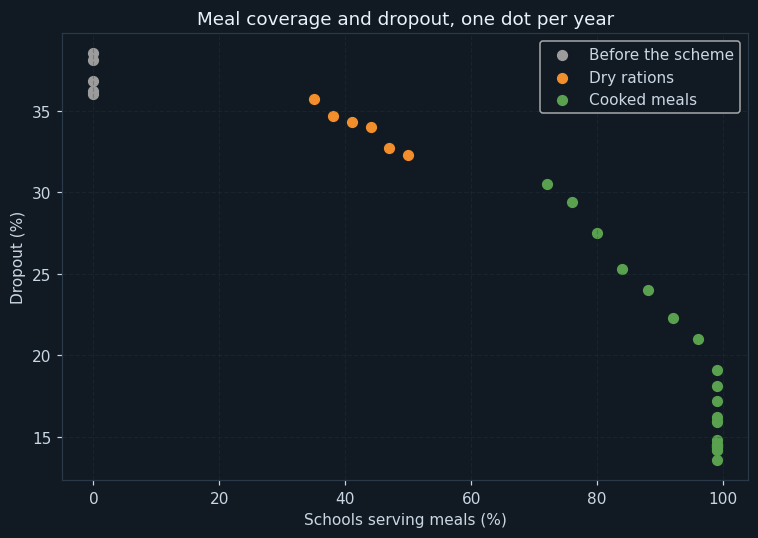
Each dot is a year: the share of schools serving meals across, dropout up, coloured by period.
The correlation is strong — -0.92 — and the three periods form three clusters. But look at the right edge: once coverage reached 99%, dropout kept falling for years and then stopped. Coverage alone cannot explain that, which is why the story must speak of contribution, not sole cause.
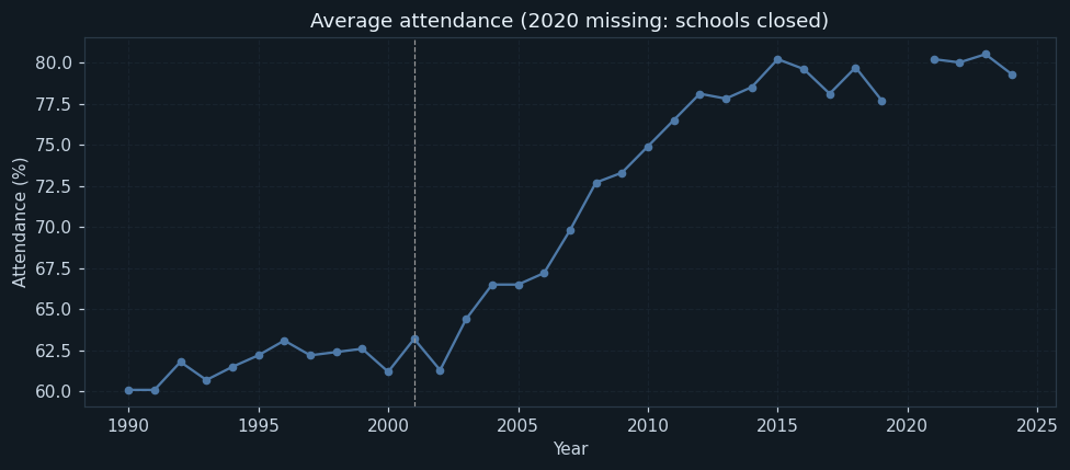
Average attendance each year. The gap at 2020 is deliberate — schools were closed.
Attendance was flat at about 61% until 2001 and then rose steadily to the high 70s. Of all the measures, attendance moves most clearly at the moment cooked meals arrived — matching what the headteacher said in the interviews about children staying after lunch.
8Step 7 — Modelling
The models here are regression models, but used diagnostically: they measure how fast dropout fell in each period, so that the change at 2001 can be tested rather than eyeballed.
The models are fitted on 1990–2019 — 30 years. The COVID years are excluded from fitting, for the reason given in Step 6.
How the models work
Model A is one straight line through all the years. Its slope is -1.02 points a year: an average fall, which assumes nothing changed in 2001.
Model B is the same Linear Regression with the two engineered features added, so its slope can change at 2001 and at 2012. It found a slope of -0.72 points a year before cooked meals, -1.59 points a year from 2001 to 2012, and 0.24 points a year afterwards. The fall more than doubled in speed when cooked meals began, then stopped. Because the fitted line must join up at each break, its last slope is slightly above zero although the plateau years are flat — a small artefact worth mentioning in a viva.
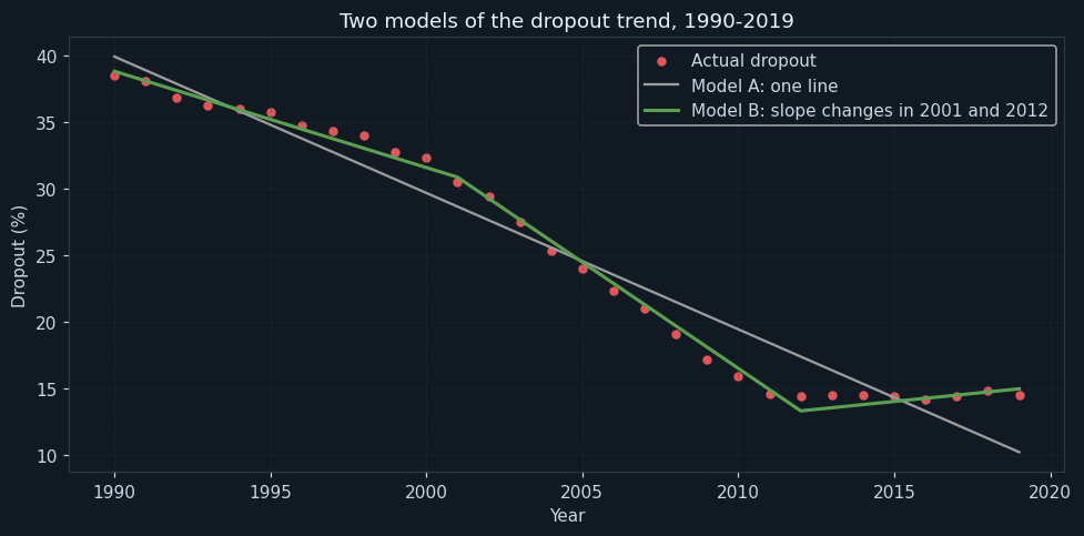
Actual dropout, 1990–2019 (dots), with Model A's single straight line and Model B's line that bends in 2001 and 2012.
Model A misses systematically: too low before 2001, too high through the 2000s, too low again after 2012. Model B follows the data closely. When a straight line's errors form a pattern like this, the line is the wrong shape — and the right shape is the evidence that something changed.
9Step 8 — Evaluation
With only thirty years, a train-test split would leave too few years to test on. The handbook's answer for small datasets is cross validation, and the strictest form is leave-one-out: each of the 30 years is held out once, the model is fitted on the other years, and the held-out year is predicted.
Model A's leave-one-out RMSE was 2.23 points; Model B's was 0.63 points — less than a third of the error. R² rises from 0.948 to 0.996. A trend that bends at 2001 and 2012 describes the data far better than a steady one.
What this proves, and what it does not. It shows that the dropout trend changed sharply when cooked meals began. It does not show that meals alone caused the change: the Sarva Shiksha Abhiyan and, later, the Right to Education Act also arrived in these years, and none of them is separated out in this data. The story must say "the fall accelerated when cooked meals arrived" — not "meals caused the fall". Saying exactly as much as the evidence supports is what makes a data story trustworthy.
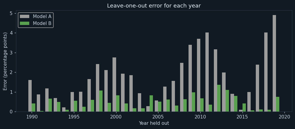
Each pair of bars is one year: the error made predicting it when that year was held out and the model fitted on all the others.
Model B's errors are small in almost every year; Model A's are large at both ends and around the break. Leave-one-out validation means each year is judged by a model that never saw it — so Model B's advantage is not just closer fitting of the same points.
10Step 9 — Deployment
For a data story, deployment means presenting it to its audience. The program writes the five beats of the story from the data itself — so every number in the story is the number in the table — and draws them on Freytag's pyramid (chart 7) and as a headline chart (chart 8).
In use, the story would be a one-page brief or a short presentation for a district review meeting: the headline chart first, the pyramid as the spoken structure, charts 2 and 4 as supporting evidence, and one slide on what the data cannot prove. The handbook's steps for building a data story — know the audience, find the insight, choose the visual, build the narrative — map onto exactly that order.
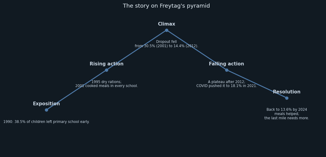
The five stages of Freytag's pyramid — the narrative structure the handbook teaches for data stories — with this story's beats under each, filled in from the data by the program.
Exposition sets the scene with the 1990 dropout rate. Rising action brings the scheme and the cooked-meal order. The climax is the steepest fall. Falling action is the plateau and the COVID shock. The resolution is the honest ending: meals helped greatly, and the last stretch needs more than meals.
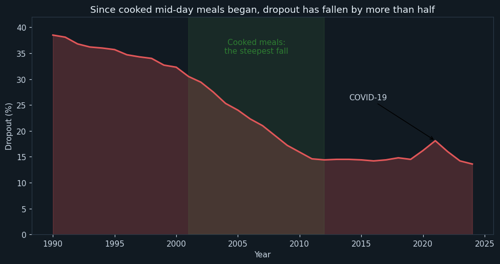
The one chart the story would lead with: dropout over time, the cooked-meal years shaded, the COVID rise labelled, and the claim in the title.
The title makes one checkable claim — dropout has fallen by more than half since cooked meals began, from 30.5% in 2001 to 13.6% in 2024 — and the chart shows it. The y-axis starts at zero: starting it at 10 would make the fall look even steeper, and that would be a misleading chart, however true the numbers.
11Step 10 — Feedback
A data story makes claims that new data can test. Its ending says dropout has returned to the plateau after COVID. The program checks that claim: the plateau years 2012–2019 averaged 14.5 %%, and the latest years average 13.9 %%.
The rule used is simple: if the latest years are within one percentage point of the plateau, the ending holds; otherwise the story must be revised. Here it holds. Each year's new figures should be run through the same check.
Feedback from the audience matters just as much. If officials ask about girls, the story gains a beat on girls' enrolment; if teachers say attendance is the better measure, the headline chart might switch to attendance. That is the methodology's loop back to Business Understanding.
12Ethical considerations
Meal coverage and dropout correlate strongly, but other programmes arrived at the same time. The story says the fall accelerated when meals arrived; it does not claim meals were the only cause. Overclaiming is the most common ethical failure in data storytelling.
The headline chart's axis starts at zero. Cutting the axis, choosing a convenient start year, or hiding the COVID rise would make the story more dramatic and less true. The handbook's ethics of data storytelling ask for accuracy over impact.
Leaving 2020's attendance blank, and saying why, is more honest than filling it — and tells the reader something real about that year.
Behind every percentage are children. A story about dropout should not blame families; the interviews show children leave for reasons of poverty, distance and safety, and the story should say so.
13Source code
The whole program, laid out as the ten steps of the methodology. Every chart and number on this page came out of running it.
# ---------------------------------------------------------------------------
# meal_story.py
#
# Capstone project: a data story about the Mid-Day Meal Scheme - how
# enrolment, attendance and dropout in one state's primary schools changed
# after the scheme began in 1995 and cooked meals arrived in 2001.
#
# CBSE Class XII, Artificial Intelligence (843), Part C - Capstone Project.
# This is the curriculum's own sample data-storytelling problem.
# SDG 4 (Quality Education) and SDG 2 (Zero Hunger).
#
# Data Science Methodology, 10 steps. The analytics is DESCRIPTIVE (what
# happened) and DIAGNOSTIC (why it may have happened). Two models of the
# dropout trend are compared with leave-one-out cross validation:
#   A. one straight line for all the years
#   B. a line allowed to change slope in 2001 and again in 2012
#      (segmented regression)
# The output of the project is a data story, structured on Freytag's pyramid.
#
# Libraries: pandas, numpy, matplotlib, scikit-learn.
# ---------------------------------------------------------------------------

# %% Step 1 - Business Understanding
print("=" * 64)
print("THE MID-DAY MEAL STORY")
print("=" * 64)
print("Question : did dropout fall after the Mid-Day Meal Scheme began,")
print("           and is the change large enough to tell a story about?")
print()

# %% Step 2 - Analytic Approach
print("Analytic approach : descriptive (what happened) and diagnostic (why)")
print()

# %% Step 3 - Data Requirements
import pandas as pd
import numpy as np
import matplotlib.pyplot as plt
from sklearn.linear_model import LinearRegression
from sklearn.model_selection import LeaveOneOut, cross_val_score

pd.set_option("display.width", 130)
pd.set_option("display.max_columns", 20)
required = ["year", "enrolment_lakh", "girls_share_pct", "attendance_pct", "dropout_pct", "meal_coverage_pct"]
print("Columns required :", required)

# %% Step 4 - Data Collection
data = pd.read_csv("school_data.csv")
print("Rows collected   :", len(data))
print("Years covered    :", data["year"].min(), "to", data["year"].max())
print()

# %% Step 5 - Data Understanding
print("--- Step 5: Data Understanding ---")
print("Missing values:")
print(data.isnull().sum().to_string())
print()
print(data.describe().round(1))
print()

events = {1995: "Scheme begins\n(dry rations)", 2001: "Cooked meals\n(court order)",
          2010: "RTE Act", 2020: "COVID-19\nclosures"}

# Chart 1: dropout over the years, with the events marked.
plt.figure(figsize=(9, 4.5))
plt.plot(data["year"], data["dropout_pct"], marker="o", color="#e15759", markersize=4)
for y in events:
    plt.axvline(y, color="#999999", linestyle="--", linewidth=0.8)
    plt.text(y + 0.3, 37, events[y], fontsize=8, va="top")
plt.title("Primary school dropout rate, 1990-2024")
plt.xlabel("Year")
plt.ylabel("Dropout (%)")
plt.grid(True, linestyle="--", alpha=0.3)
plt.tight_layout()
plt.savefig("chart1_dropout.png")
plt.close()

# Chart 2: enrolment and the share of girls.
plt.figure(figsize=(10, 4))
plt.subplot(1, 2, 1)
plt.plot(data["year"], data["enrolment_lakh"], color="#4e79a7")
plt.title("Enrolment (lakh children)")
plt.xlabel("Year")
plt.grid(True, linestyle="--", alpha=0.3)
plt.subplot(1, 2, 2)
plt.plot(data["year"], data["girls_share_pct"], color="#b07aa1")
plt.title("Girls as % of enrolment")
plt.xlabel("Year")
plt.grid(True, linestyle="--", alpha=0.3)
plt.tight_layout()
plt.savefig("chart2_enrolment.png")
plt.close()

# %% Step 6 - Data Preparation
print("--- Step 6: Data Preparation ---")
before = len(data)
data = data.drop_duplicates()
print("Duplicate rows removed       :", before - len(data))

# Attendance is missing for 1998 (records lost) and 2020 (schools closed).
# 1998 is filled by linear interpolation between 1997 and 1999. 2020 is
# left empty on purpose: there was no attendance to record, and inventing
# a value would hide the most important fact about that year.
data["attendance_pct"] = pd.to_numeric(data["attendance_pct"])
data.loc[data["year"] == 1998, "attendance_pct"] = np.nan
filled = data["attendance_pct"].interpolate()
data.loc[data["year"] == 1998, "attendance_pct"] = filled[data["year"] == 1998]
print("Attendance 1998 (interpolated) :", round(data.loc[data["year"] == 1998, "attendance_pct"].values[0], 1))
print("Attendance 2020                 : left missing - schools were closed")

# Feature engineering: the period each year belongs to.
period = []
for y in data["year"]:
    if y < 1995:
        period.append("Before the scheme")
    elif y < 2001:
        period.append("Dry rations")
    else:
        period.append("Cooked meals")
data["period"] = period
# Chart 1 shows the fall steepening in 2001 and flattening around 2012, so
# two "years since" features let a straight-line model bend at both points.
data["years_since_2001"] = np.maximum(0, data["year"] - 2001)
data["years_since_2012"] = np.maximum(0, data["year"] - 2012)
print()

summary = data.groupby("period", sort=False)[["dropout_pct", "attendance_pct", "enrolment_lakh"]].mean().round(1)
print("Average of each period:")
print(summary)
print()
print("Average dropout before the scheme :", summary.loc["Before the scheme", "dropout_pct"], "%")
print("Average dropout with cooked meals :", summary.loc["Cooked meals", "dropout_pct"], "%")
print()

corr_cov = data["meal_coverage_pct"].corr(data["dropout_pct"])
corr_att = data["meal_coverage_pct"].corr(data["attendance_pct"])
print("Correlation, meal coverage and dropout    :", round(corr_cov, 2))
print("Correlation, meal coverage and attendance :", round(corr_att, 2))
print()

# Chart 3: meal coverage against dropout, coloured by period.
colours = {"Before the scheme": "#9c9c9c", "Dry rations": "#f28e2b", "Cooked meals": "#59a14f"}
plt.figure(figsize=(7, 5))
for p in colours:
    part = data[data["period"] == p]
    plt.scatter(part["meal_coverage_pct"], part["dropout_pct"], color=colours[p], label=p, s=40)
plt.title("Meal coverage and dropout, one dot per year")
plt.xlabel("Schools serving meals (%)")
plt.ylabel("Dropout (%)")
plt.legend()
plt.grid(True, linestyle="--", alpha=0.3)
plt.tight_layout()
plt.savefig("chart3_coverage_dropout.png")
plt.close()

# Chart 4: attendance, with the 2020 gap visible.
plt.figure(figsize=(9, 4))
plt.plot(data["year"], data["attendance_pct"], marker="o", markersize=4, color="#4e79a7")
plt.axvline(2001, color="#999999", linestyle="--", linewidth=0.8)
plt.title("Average attendance (2020 missing: schools closed)")
plt.xlabel("Year")
plt.ylabel("Attendance (%)")
plt.grid(True, linestyle="--", alpha=0.3)
plt.tight_layout()
plt.savefig("chart4_attendance.png")
plt.close()

# %% Step 7 - Modelling
print("--- Step 7: Modelling ---")
# The trend is modelled on 1990-2019. 2020-2024 are left out of the fit:
# COVID-19 was an outside shock that no school-meal model should explain.
trend = data[data["year"] <= 2019]
y = trend["dropout_pct"]
X_a = trend[["year"]]
X_b = trend[["year", "years_since_2001", "years_since_2012"]]
model_a = LinearRegression().fit(X_a, y)
model_b = LinearRegression().fit(X_b, y)
print("Model A slope (all years)            :", round(model_a.coef_[0], 2), "points a year")
slope_before = model_b.coef_[0]
slope_meals = model_b.coef_[0] + model_b.coef_[1]
slope_plateau = slope_meals + model_b.coef_[2]
print("Model B slope before 2001            :", round(slope_before, 2), "points a year")
print("Model B slope 2001 to 2012           :", round(slope_meals, 2), "points a year")
print("Model B slope after 2012             :", round(slope_plateau, 2), "points a year")
print()

# %% Step 8 - Evaluation
print("--- Step 8: Evaluation ---")
# Leave-one-out cross validation: each year in turn is held out, the model
# is fitted on the other years, and the held-out year is predicted.
loo = LeaveOneOut()
err_a = np.sqrt(-cross_val_score(LinearRegression(), X_a, y, cv=loo, scoring="neg_mean_squared_error"))
err_b = np.sqrt(-cross_val_score(LinearRegression(), X_b, y, cv=loo, scoring="neg_mean_squared_error"))
rmse_a = np.sqrt((err_a ** 2).mean())
rmse_b = np.sqrt((err_b ** 2).mean())
print("Years used for the trend          :", len(trend))
print("Leave-one-out RMSE, Model A       :", round(rmse_a, 2), "points")
print("Leave-one-out RMSE, Model B       :", round(rmse_b, 2), "points")
print("R squared, Model A                :", round(model_a.score(X_a, y), 3))
print("R squared, Model B                :", round(model_b.score(X_b, y), 3))
print()

# Chart 5: the two trend models over the data.
plt.figure(figsize=(9, 4.5))
plt.scatter(trend["year"], y, color="#e15759", s=20, label="Actual dropout")
plt.plot(trend["year"], model_a.predict(X_a), color="#9c9c9c", label="Model A: one line")
plt.plot(trend["year"], model_b.predict(X_b), color="#59a14f", linewidth=2, label="Model B: slope changes in 2001 and 2012")
plt.title("Two models of the dropout trend, 1990-2019")
plt.xlabel("Year")
plt.ylabel("Dropout (%)")
plt.legend()
plt.grid(True, linestyle="--", alpha=0.3)
plt.tight_layout()
plt.savefig("chart5_models.png")
plt.close()

# Chart 6: leave-one-out error for each year.
plt.figure(figsize=(9, 4))
plt.bar(trend["year"] - 0.2, err_a, width=0.4, color="#9c9c9c", label="Model A")
plt.bar(trend["year"] + 0.2, err_b, width=0.4, color="#59a14f", label="Model B")
plt.title("Leave-one-out error for each year")
plt.xlabel("Year held out")
plt.ylabel("Error (percentage points)")
plt.legend()
plt.tight_layout()
plt.savefig("chart6_loo_errors.png")
plt.close()

# %% Step 9 - Deployment
print("--- Step 9: Deployment: the data story ---")
d_1990 = data.loc[data["year"] == 1990, "dropout_pct"].values[0]
d_2001 = data.loc[data["year"] == 2001, "dropout_pct"].values[0]
d_2012 = data.loc[data["year"] == 2012, "dropout_pct"].values[0]
d_2021 = data.loc[data["year"] == 2021, "dropout_pct"].values[0]
d_2024 = data.loc[data["year"] == 2024, "dropout_pct"].values[0]
story = [
    ["Exposition", "1990: " + str(d_1990) + "% of children left primary school early."],
    ["Rising action", "1995 dry rations; 2001 cooked meals in every school."],
    ["Climax", "Dropout fell from " + str(d_2001) + "% (2001) to " + str(d_2012) + "% (2012)."],
    ["Falling action", "A plateau after 2012; COVID pushed it to " + str(d_2021) + "% in 2021."],
    ["Resolution", "Back to " + str(d_2024) + "% by 2024 - meals helped; the last mile needs more."],
]
for stage, beat in story:
    print(stage.ljust(15), ":", beat)
print()

# Chart 7: Freytag's pyramid, carrying this story's beats.
xs = [0, 1, 2, 3, 4]
ys = [0, 1, 2, 1, 0.3]
plt.figure(figsize=(10, 4.8))
plt.plot(xs, ys, color="#4e79a7", marker="o", linewidth=2)
for i in range(5):
    plt.text(xs[i], ys[i] + 0.12, story[i][0], ha="center", fontsize=10, fontweight="bold")
    plt.text(xs[i], ys[i] - 0.25, story[i][1].replace("; ", ";\n").replace(" from", "\nfrom").replace(" - ", "\n"),
             ha="center", fontsize=7.5, va="top")
plt.ylim(-1.1, 2.5)
plt.xlim(-0.6, 4.6)
plt.axis("off")
plt.title("The story on Freytag's pyramid")
plt.tight_layout()
plt.savefig("chart7_freytag.png")
plt.close()

# Chart 8: the headline chart of the story.
plt.figure(figsize=(9, 4.8))
plt.fill_between(data["year"], data["dropout_pct"], color="#e15759", alpha=0.25)
plt.plot(data["year"], data["dropout_pct"], color="#e15759", linewidth=2)
plt.axvspan(2001, 2012, color="#59a14f", alpha=0.12)
plt.text(2006.5, 35, "Cooked meals:\nthe steepest fall", ha="center", fontsize=10, color="#2e7d32")
plt.annotate("COVID-19", xy=(2021, d_2021), xytext=(2014, 26), arrowprops=dict(arrowstyle="->"))
plt.title("Since cooked mid-day meals began, dropout has fallen by more than half")
plt.xlabel("Year")
plt.ylabel("Dropout (%)")
plt.ylim(0, 42)
plt.tight_layout()
plt.savefig("chart8_headline.png")
plt.close()

# %% Step 10 - Feedback
print("--- Step 10: Feedback ---")
# The story makes a claim that new data can test: dropout should stay near
# the post-2012 plateau. Model B's plateau-era average is compared with the
# years after COVID as they arrive.
plateau = data[(data["year"] >= 2012) & (data["year"] <= 2019)]["dropout_pct"].mean()
latest = data[data["year"] >= 2023]["dropout_pct"].mean()
print("Average dropout 2012-2019 (plateau) :", round(plateau, 1), "%")
print("Average dropout 2023-2024 (latest)  :", round(latest, 1), "%")
if abs(latest - plateau) <= 1.0:
    print("Feedback: the latest years are back on the plateau - the story's ending holds.")
else:
    print("Feedback: the latest years differ from the plateau - the story's ending must be revised.")
The library calls it is built from
| Call | Step | What it does |
|---|---|---|
pd.read_csv() / describe() | Steps 4–5 | Reads the data and summarises it |
drop_duplicates() | Step 6 | Removes the repeated year |
Series.interpolate() | Step 6 | Fills 1998's attendance from its neighbours |
groupby("period").mean() | Step 6 | Averages for each period |
Series.corr() | Step 6 | Correlation of meal coverage with dropout and attendance |
np.maximum(0, year - 2001) | Step 6 | Engineered feature: years since a break point |
LinearRegression().fit() | Step 7 | Fits Model A and Model B |
LeaveOneOut() + cross_val_score() | Step 8 | Leave-one-out cross validation |
plt.axvline / axvspan / annotate | Steps 5, 9 | Marks events, shades a period, labels a point on the story charts |
14Output of a real run
================================================================
THE MID-DAY MEAL STORY
================================================================
Question : did dropout fall after the Mid-Day Meal Scheme began,
           and is the change large enough to tell a story about?

Analytic approach : descriptive (what happened) and diagnostic (why)

Columns required : ['year', 'enrolment_lakh', 'girls_share_pct', 'attendance_pct', 'dropout_pct', 'meal_coverage_pct']
Rows collected   : 36
Years covered    : 1990 to 2024

--- Step 5: Data Understanding ---
Missing values:
year                 0
enrolment_lakh       0
girls_share_pct      0
attendance_pct       2
dropout_pct          0
meal_coverage_pct    0

         year  enrolment_lakh  girls_share_pct  attendance_pct  dropout_pct  meal_coverage_pct
count    36.0            36.0             36.0            34.0         36.0               36.0
mean   2007.0            55.1             47.1            70.3         23.6               72.8
std      10.1             9.5              2.5             7.8          9.1               36.1
min    1990.0            40.8             43.4            60.1         13.6                0.0
25%    1998.8            46.0             44.6            62.3         14.6               46.2
50%    2007.0            55.3             47.3            69.8         21.0               96.0
75%    2015.2            64.1             49.4            78.1         33.0               99.0
max    2024.0            68.9             50.4            80.5         38.5               99.0

--- Step 6: Data Preparation ---
Duplicate rows removed       : 1
Attendance 1998 (interpolated) : 62.4
Attendance 2020                 : left missing - schools were closed

Average of each period:
                   dropout_pct  attendance_pct  enrolment_lakh
period
Before the scheme         37.1            60.8            42.1
Dry rations               33.9            62.3            45.1
Cooked meals              18.4            74.2            60.3

Average dropout before the scheme : 37.1 %
Average dropout with cooked meals : 18.4 %

Correlation, meal coverage and dropout    : -0.92
Correlation, meal coverage and attendance : 0.82

--- Step 7: Modelling ---
Model A slope (all years)            : -1.02 points a year
Model B slope before 2001            : -0.72 points a year
Model B slope 2001 to 2012           : -1.59 points a year
Model B slope after 2012             : 0.24 points a year

--- Step 8: Evaluation ---
Years used for the trend          : 30
Leave-one-out RMSE, Model A       : 2.23 points
Leave-one-out RMSE, Model B       : 0.63 points
R squared, Model A                : 0.948
R squared, Model B                : 0.996

--- Step 9: Deployment: the data story ---
Exposition      : 1990: 38.5% of children left primary school early.
Rising action   : 1995 dry rations; 2001 cooked meals in every school.
Climax          : Dropout fell from 30.5% (2001) to 14.4% (2012).
Falling action  : A plateau after 2012; COVID pushed it to 18.1% in 2021.
Resolution      : Back to 13.6% by 2024 - meals helped; the last mile needs more.

--- Step 10: Feedback ---
Average dropout 2012-2019 (plateau) : 14.5 %
Average dropout 2023-2024 (latest)  : 13.9 %
Feedback: the latest years are back on the plateau - the story's ending holds.15The same project in Orange
The descriptive half of this project is natural in Orange, and its visualisation widgets can produce the story's charts. The tool is Orange Data Mining.
| Widget | What it does |
|---|---|
| File | Load school_data.csv. |
| Data Table + Feature Statistics | Find the duplicate and the two missing attendance values. |
| Impute | Interpolate or set a value for 1998; leave 2020 missing by excluding that row from attendance analysis. |
| Feature Constructor | Make the period column and the years_since features. |
| Line Plot / Scatter Plot | Draw dropout over the years and coverage against dropout. |
| Linear Regression + Test and Score | Compare the one-line and segmented models with Leave-one-out validation. |
| Report | Collect the charts and notes into a report — the start of the data story. |
16Testing
Every case was run: each gives the whole program a small input of its own.
| Test case | Expected | Actual | Result |
|---|---|---|---|
| All rows read, 1990 to 2024 | Years covered : 1990 to 2024 | Years covered : 1990 to 2024 | Pass |
| The 2007 row entered twice is removed | Duplicate rows removed : 1 | Duplicate rows removed : 1 | Pass |
| Attendance for 1998 is interpolated from 1997 and 1999 | Attendance 1998 (interpolated) : 62.4 | Attendance 1998 (interpolated) : 62.4 | Pass |
| Attendance for 2020 is deliberately left missing | Attendance 2020 : left missing - schools were closed | Attendance 2020 : left missing - schools were closed | Pass |
| Bending the line in 2001 and 2012 cuts the leave-one-out error | Leave-one-out RMSE, Model B : 0.63 points | Leave-one-out RMSE, Model B : 0.63 points | Pass |
| Dropout falling exactly 1 point a year: Model A's slope is -1 | Model A slope (all years) : -1.0 points a year | Model A slope (all years) : -1.0 points a year | Pass |
| A trend that bends exactly in 2001: Model B finds the -2.0 slope | Model B slope 2001 to 2012 : -2.0 points a year | Model B slope 2001 to 2012 : -2.0 points a year | Pass |
| ...and the flat-ish slope after 2012 | Model B slope after 2012 : 0.0 points a year | Model B slope after 2012 : 0.0 points a year | Pass |
| The data file is missing | FileNotFoundError: [Errno 2] No such file or directory: 'school_data.csv' | FileNotFoundError: [Errno 2] No such file or directory: 'school_data.csv' | Pass |
17Team roles and timeline
A capstone is done by a group of 3 to 5. A suggested split of the work, and a timeline across the year:
| Role | Responsible for |
|---|---|
| Project lead | Business understanding, interviews with teachers and officials, the final presentation |
| Data lead | Finding and downloading UDISE+ and scheme data for the state; recording sources |
| Analyst | Data understanding and preparation; the period comparisons and correlations |
| Modeller | The two trend models and leave-one-out validation |
| Storyteller | The Freytag structure, the headline chart, the written brief and the 3-minute video |
| When | Methodology steps | Deliverable |
|---|---|---|
| April – May | 1 Business Understanding, 2 Analytic Approach | Question and 5W1H canvas; interviews |
| June – July | 3 Data Requirements, 4 Data Collection | State data downloaded; event dates verified |
| August | 5 Data Understanding, 6 Data Preparation | Clean series; first charts |
| September – October | 7 Modelling, 8 Evaluation | Trend models compared |
| November | 9 Deployment, 10 Feedback | Story drafted; presented to the class for feedback |
| December – January | Documentation and video | Report and 3-minute video |
18Results, limits and what next
- Average dropout fell from 37.1 % before the scheme to 18.4 % in the cooked-meal years.
- The fall more than doubled in speed when cooked meals began — from -0.72 points a year to -1.59 points a year points a year — and then levelled off after 2012.
- A trend that bends at 2001 and 2012 fits far better than one straight line: leave-one-out RMSE 0.63 points against 2.23 points.
- Attendance rose most clearly at the moment cooked meals arrived; enrolment and the girls' share rose too.
- The data shows the change, not its sole cause — other programmes arrived in the same years.
Limitations
- Sample data for an imaginary state; real state figures will differ
- Other programmes (SSA, RTE) are not separated out, so causation cannot be claimed
- State averages hide differences between districts, and between boys and girls
- Only thirty years for the trend models — enough to show a change, not to model it finely
Future scope
- Use real UDISE+ data for your own state and district
- Compare a state that adopted cooked meals early with one that adopted late — a natural experiment
- Add girls' dropout separately and tell the girls' story
- Add nutrition outcomes, such as the share of underweight children, for the SDG 2 side
What the team had to learn
- Freytag's pyramid and the steps to create a story through data
- Diagnostic analytics: what correlation can and cannot show
- Segmented regression built with engineered features
- Leave-one-out cross validation for small datasets
19Conclusion
The capstone told the curriculum's sample data story and tested it. Dropout fell throughout the period, but the fall accelerated sharply when cooked meals arrived in 2001 and levelled off after 2012 — a pattern a segmented regression captures far better than a single line, as leave-one-out validation confirms.
The most important part of the story is what it leaves out. The data cannot separate the scheme from the other changes of the same years, and an honest data story says so. A claim the evidence supports exactly is worth more than a dramatic one that collapses when questioned.
Freytag's pyramid turned thirty-five rows of numbers into something an official, a parent or a journalist can follow in a minute — which is the whole purpose of data storytelling.
20The 3-minute video script
Part C asks for a video of exactly three minutes with six parts. A script, timed to the second:
| Time | Part | What to say and show |
|---|---|---|
| 0:00 – 0:25 | a. Problem statement | Show children eating a mid-day meal. "Has the Mid-Day Meal Scheme kept children in school? The numbers exist — but nobody reads thirty-five years of tables." |
| 0:25 – 0:45 | b. SDG alignment | SDG 4 and SDG 2 icons. "A meal at school feeds a child and keeps that child in class." |
| 0:45 – 1:15 | c. AI concepts and algorithms | "Descriptive and diagnostic analytics. We compared a single trend line with a segmented regression using leave-one-out cross validation, and told the result on Freytag's pyramid." |
| 1:15 – 2:20 | d. How it works | Walk up Freytag's pyramid (chart 7), stage by stage, showing chart 1 for the exposition, chart 5 for the climax and the COVID bump for the falling action. Show the validation numbers. |
| 2:20 – 2:45 | e. Conclusion | Headline chart (chart 8). "Dropout has fallen by more than half since cooked meals began. Meals helped — and the data cannot say they did it alone." |
| 2:45 – 3:00 | f. Acknowledgement | "We thank our AI teacher, [name], and the teachers and officers who spoke to us." |
21Questions for the viva
▸What type of analytics is your project?
Descriptive, because it summarises what happened in each period, and diagnostic, because it tests whether the dropout trend changed when cooked meals began.
▸Why did you treat the two missing attendance values differently?
1998's records were lost, so interpolating between 1997 and 1999 gives a fair estimate. In 2020 schools were closed, so there was no attendance; filling it would hide a real fact.
▸What is segmented regression, and how did you build it?
A regression whose slope can change at chosen points. We added two features — years since 2001 and years since 2012 — to an ordinary Linear Regression.
▸Why leave-one-out cross validation?
We had only thirty years. Leave-one-out uses every year for testing once while training on all the others, which is the most reliable option for a small dataset.
▸Does your project prove the scheme reduced dropout?
No. It shows the fall accelerated when cooked meals began, but other programmes arrived in the same years, so we cannot claim meals were the only cause.
▸What are the stages of Freytag's pyramid?
Exposition, rising action, climax, falling action and resolution.
▸Why does your headline chart start its axis at zero?
Starting higher would exaggerate the fall. Honest charts are part of the ethics of data storytelling.
▸Which SDGs does it align to?
SDG 4, Quality Education, and SDG 2, Zero Hunger.
22References
- Ministry of Education, Government of India — PM POSHAN (formerly Mid-Day Meal Scheme) — https://pmposhan.education.gov.in/
- UDISE+, Ministry of Education — school enrolment and dropout data — https://udiseplus.gov.in/
- People's Union for Civil Liberties v. Union of India, Supreme Court order of 28 November 2001 (cooked mid-day meals).
- The Right of Children to Free and Compulsory Education Act, 2009 (in force 1 April 2010).
- Freytag, G. (1863). Die Technik des Dramas — the source of Freytag's pyramid.
- CBSE, Artificial Intelligence (Subject Code 843), Class XII curriculum, 2026-27 — Part C
- CBSE, Artificial Intelligence Student Handbook, Class XII — Unit 2, Data Science Methodology
- Rollins, J. B. (2015). Foundational Methodology for Data Science. IBM Analytics.
- scikit-learn — https://scikit-learn.org/stable/; pandas, NumPy and Matplotlib documentation
- LambdaLab — https://www.lambdalab.in