Spotting Coral Bleaching
The curriculum's own Computer Vision project: reading reef photos pixel by pixel to tell healthy coral from bleached.
1Introduction
Divers and underwater drones take thousands of photos of a reef on every survey. A scientist then has to look at each one and decide: is this coral healthy or bleached?
That takes weeks, and by the time the photos are sorted the bleaching may have spread. The colour of the coral is the main clue, and colour is something a computer can measure exactly.
This is the Computer Vision sample project in the CBSE curriculum, which builds it in Orange Data Mining. Here it is built in Python, so that every step — from pixels to prediction — can be seen.
Life below Water
Climate Action
Coral reefs are home to about a quarter of all sea life, though they cover a tiny part of the ocean. When the sea gets too warm, corals push out the tiny algae that live in them and give them colour, and turn white — this is bleaching. A bleached coral can recover if the water cools in time, but repeated bleaching kills reefs. Finding it early tells scientists where reefs need protection, which is SDG 14; the warming behind it is SDG 13.
The curriculum asks that the project be related to the Sustainable Development Goals. That link is the reason the problem is worth solving, so it belongs at the very start of the report, not tacked on at the end.
2Stage 1 — Problem Scoping
Problem scoping means understanding the problem properly before building anything. The tool for it is the 4Ws Problem Canvas: who has the problem, what the problem is, where it happens, and why solving it matters.
- Marine scientists studying coral reefs
- Divers and reef-protection groups who take the photos
- Thousands of reef photos are too many to check by eye quickly
- Bleaching found late may be too late to protect a reef
- Coral reefs, such as Lakshadweep and the Gulf of Mannar
- After each survey dive, especially in hot summers
- Bleached areas can be found and protected sooner
- Scientists' time goes to the reefs that need it
The problem statement
The four answers are then joined into one sentence, using the curriculum's problem statement template:
Marine scientists and trained divers who photograph reefs, such as those around Lakshadweep, the Andaman and Nicobar Islands and the Gulf of Mannar.
How it is done today
Accurate, but very slow. A single survey can take weeks to sort.
Divers hold a card of coral colours up to the reef and note the closest match. Clever and cheap, but done by hand, one coral at a time.
Satellites warn when the sea is hot enough to cause bleaching. They predict the risk; they cannot see whether a particular coral has actually bleached.
Objectives
- To read reef photos into Python as arrays of pixel values
- To see how a colour photo is stored as red, green and blue layers
- To separate coral pixels from water pixels
- To measure two features of the coral — brightness and colourfulness — from every photo
- To build a model that learns the average healthy and bleached coral, and test it on unseen photos
- To look at the photos it got wrong and understand why
- To label new photos from a survey
📘 Revise: Stage 1 — Problem Scoping
3Stage 2 — Data Acquisition
The data is a folder of photos, one folder for each class: images/healthy/ and images/bleached/. This is the same layout that Teachable Machine and Orange use.
There are 160 photos, each 64 × 64 pixels. A second folder, new_photos/, holds four photos from a new survey that the model has never seen.
These pictures were drawn by a program, not taken in the sea, so that the project can be shared freely and run anywhere. The curriculum's own coral dataset (linked from the CBSE curriculum) uses real photos. For your project, use that dataset or another public one, and credit it — never present drawn pictures as real reef photos.
Features and label
The features are what the model is given. The label is the answer it has to learn to give.
| Column | Type | What it holds | Role |
|---|---|---|---|
brightness | decimal | Average of the coral pixels' R, G and B values (0 = black, 255 = white) | feature |
colourfulness | decimal | Average gap between each coral pixel's largest and smallest colour value (0 = grey or white) | feature |
label | text | healthy or bleached — the folder the photo came from | label |
photo | file | The photo, read as a 64 × 64 × 3 array of numbers | not used |
coral_pixels | integer | How many pixels were counted as coral | not used |
Inside the images/ folder
Reef photos sorted into a healthy folder and a bleached folder. Lighting and the blue cast of deep water change from photo to photo, and some corals are part-way, so the job is not trivially easy. There are 160 images, 1393.8 KB in all, one folder per class — the same layout Teachable Machine and Orange expect:
The images come with the project download.
Inside the new_photos/ folder
Four photos from a new survey, used in the deployment stage. There are 4 images, 34.8 KB in all.
The images come with the project download.
📘 Revise: Stage 2 — Data Acquisition
4Stage 3 — Data Exploration
Data exploration means getting to know the data before trusting it: fixing what is wrong with it, then drawing it to see the patterns. The charts here are what decide what the model should be.
What was wrong with the data
Averaging the whole photo would mostly measure the water. So the program first finds the coral: water has very little red, coral has a lot, so a pixel with red above 77 (out of 255) counts as coral. Deciding which pixels belong to the object is called segmentation.
Deep or cloudy water makes everything darker and bluer. This is why the project measures colourfulness as well as brightness: a dim white coral is still grey, not brown.
Too many for a simple model to use directly. Feature extraction turns each photo into just two numbers that describe what matters — how bright and how colourful the coral is.
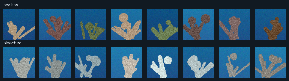
The top row is healthy coral; the bottom row is bleached. They were read from the folders with plt.imread() and shown with plt.imshow() — the practical-file program "read an image and display it using Python".
To our eyes the difference is colour: healthy coral is brown, olive or orange, and bleached coral is white or grey. But some healthy corals are pale and some bleached ones still have a little colour, and dim lighting makes everything look darker. The model will find those photos hardest.
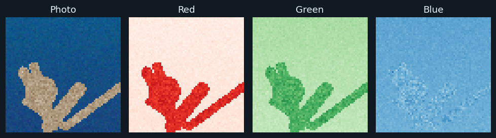
The same photo four times: as we see it, then each of its three colour layers on its own. In each layer, a darker colour means a bigger number.
This is how the computer stores a colour photo: three grids of numbers, one each for red, green and blue. The water is strong in blue and weak in red. The coral is strong in red. That one difference is what lets the program separate coral from water.
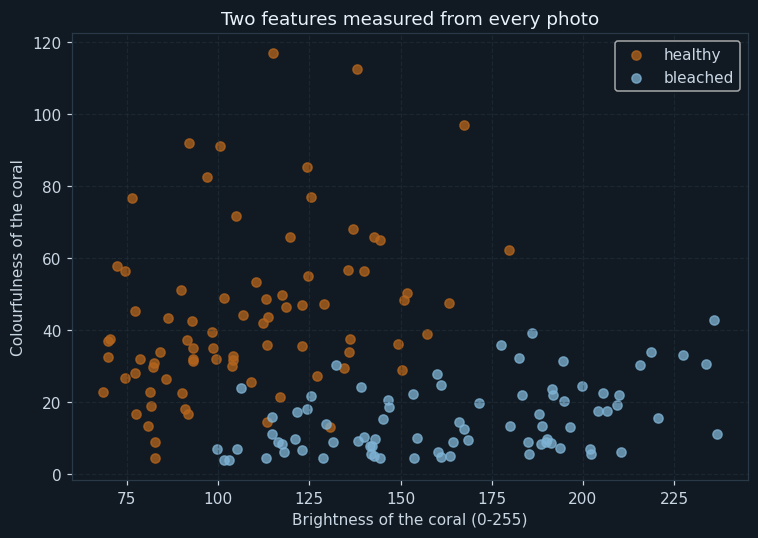
Each dot is one photo: how bright its coral is (across) and how colourful (up).
The two kinds form two clouds. Healthy coral sits up and to the left — colourful and darker. Bleached coral sits low and to the right — grey or white, and brighter. Where they meet, dim bleached corals sit close to pale healthy ones. That overlap is where the mistakes will be.
📘 Revise: Stage 3 — Data Exploration
5Stage 4 — Modelling
Where this model sits in the family of AI models:
The answer is one of two classes — healthy or bleached — so this is classification. Every training photo comes from a labelled folder, so it is supervised learning. Because the input is images, it belongs to the Computer Vision domain.
How the model works
The photos are shuffled and split into 128 for training and 32 for testing.
Each photo has already been turned into two features. The model learns the average brightness and colourfulness of healthy coral, and the same for bleached coral, from the training photos. To label a new photo, it measures the photo's two features and picks whichever average is closer.
This is the classic way computer vision worked before deep learning: a person decides which features matter (here, colour) and writes code to measure them. A Convolutional Neural Network, from Unit 5, learns its own features from the pixels instead. That is what Teachable Machine and Orange's Image Embedding do behind the scenes.
📘 Revise: Stage 4 — Modelling
6Stage 5 — Evaluation
On 32 testing photos the model reached an accuracy of 84.4 %.
For bleaching, the costly mistake is a missed bleached coral (a false negative): a reef that needs help goes unnoticed. A false alarm only means a scientist looks at one extra photo. So recall matters most. The recall was 75.0 % and the precision 100.0 %.
That recall is the honest weak point of this model. The mistakes chart shows why: dimly lit bleached corals look darker and slightly coloured. A better feature — for example, comparing the coral's colour with the colour of the water around it, to cancel out the lighting — is the obvious next step.
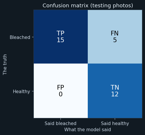
Bleached is the positive class, because it is what the scientists are looking for. TP: bleached, and found. FN: bleached, but called healthy. FP: healthy, but called bleached. TN: healthy, and called healthy.
On the testing photos the counts are 15 5 0 12 (TP, FN, FP, TN). The model never raised a false alarm, but it missed some bleached coral.
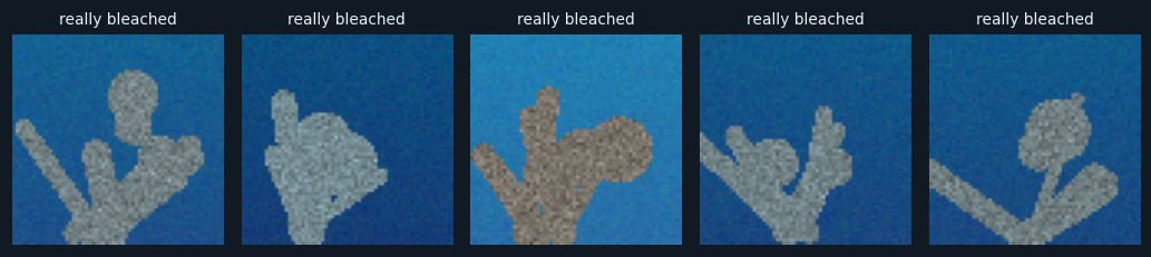
Every testing photo the model labelled wrongly, with its true label.
All the mistakes are bleached corals that it called healthy, and they have something in common: they are dimly lit, with brightness between about 115 and 130, and they still carry a little colour. In dark water, a bleached coral is not bright white any more. Looking at the mistakes tells you exactly what to fix next — which a single accuracy number never does.
📘 Revise: The Confusion Matrix
7Stage 6 — Deployment
The program reads four new survey photos it has never seen, measures their features, and labels each one. It saves them with their labels as a picture.
In real use, a scientist would point the program at a whole folder of survey photos and get back a list of the ones labelled bleached, to check first. The program does the sorting; the scientist does the judging.
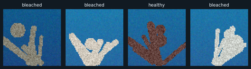
The four new photos, each with the label the model gave it.
Three are labelled correctly. The first was drawn as a healthy but very pale coral, and the model calls it bleached. That is a false alarm — but in a real reef, a coral that has gone pale is often starting to bleach, so it is exactly the photo a scientist would want to look at anyway.
📘 Revise: Stage 6 — Deployment
8Ethical concerns
An AI project is not finished when the model works. The curriculum asks three questions of every model — is it fair (bias), can it explain itself (transparency), and who answers for its mistakes (accountability). For this project:
Real reef photos belong to the scientists or divers who took them. Use public datasets, credit them, and never present drawn or edited pictures as real survey photos.
A model trained on one reef, in one kind of water, may fail on another — different coral species, different water colour. It must be tested on photos from the reef where it will be used.
A missed bleaching event could mean a reef is not protected in time. The model should help scientists check faster, not replace their checking.
📘 Revise: Bias, Transparency, Accountability
9Source code
The whole program — it is also in the downloads at the top of this page — in Python with pandas, NumPy and matplotlib — the three libraries of Unit 7. It is laid out as the six stages of the AI Project Cycle, one after another. Every chart on this page was drawn by it, and every number came out of running it.
# ---------------------------------------------------------------------------
# coral_bleaching.py
#
# AI project on Computer Vision: telling healthy coral from bleached coral in
# underwater photographs, so that bleaching can be spotted early.
#
# CBSE Class X, Artificial Intelligence (417), Part C project work.
# SDG 14 (Life below Water) and SDG 13 (Climate Action).
#
# A computer sees a photo as a grid of pixels, and each pixel as three
# numbers from 0 to 255 - how much red, green and blue it holds. The program:
#   1. reads every photo into those numbers,
#   2. finds which pixels are coral and which are water (segmentation),
#   3. measures two FEATURES of the coral: how bright it is, and how
#      colourful it is, and
#   4. learns the average healthy coral and the average bleached coral from
#      the training photos, and labels a new photo by whichever it is closer to.
#
# Libraries: numpy (the pixel arithmetic), matplotlib (reading and showing
# images, and the charts), pandas (the table of features), os (the folders).
# ---------------------------------------------------------------------------

# %% Stage 1 - Problem scoping
print("=" * 60)
print("SPOTTING CORAL BLEACHING")
print("=" * 60)
print("Who   : marine scientists and reef divers")
print("What  : thousands of reef photos, too many to check by eye")
print("Where : coral reefs, such as those around Lakshadweep")
print("Why   : bleaching caught early shows where reefs need protection")
print()

# %% Stage 2 - Data acquisition
import os
import numpy as np
import pandas as pd
import matplotlib.pyplot as plt

pd.set_option("display.width", 120)

classes = ["healthy", "bleached"]
paths = []
labels = []
for c in classes:
    for name in sorted(os.listdir(os.path.join("images", c))):
        paths.append(os.path.join("images", c, name))
        labels.append(c)

print("--- Stage 2: Data acquisition ---")
print("Healthy photos  :", labels.count("healthy"))
print("Bleached photos :", labels.count("bleached"))
print("Total photos    :", len(paths))

# Read one photo and look at what the computer actually sees.
first = plt.imread(paths[0])
print("One photo is stored as an array of shape :", first.shape)
print("Height x width x colours                 : 64 x 64 x 3 = 12288 numbers")
pixel = (first[40, 32] * 255).round()
print("The pixel at row 40, column 32 (R, G, B) :", int(pixel[0]), int(pixel[1]), int(pixel[2]))
print()

# Chart 1: eight photos of each kind, spread through each folder.
healthy_paths = []
bleached_paths = []
for i in range(len(paths)):
    if labels[i] == "healthy":
        healthy_paths.append(paths[i])
    else:
        bleached_paths.append(paths[i])
plt.figure(figsize=(9, 2.6))
for i in range(8):
    plt.subplot(2, 8, i + 1)
    plt.imshow(plt.imread(healthy_paths[i * len(healthy_paths) // 8]))
    plt.axis("off")
    if i == 0:
        plt.title("healthy", fontsize=9, loc="left")
    plt.subplot(2, 8, i + 9)
    plt.imshow(plt.imread(bleached_paths[i * len(bleached_paths) // 8]))
    plt.axis("off")
    if i == 0:
        plt.title("bleached", fontsize=9, loc="left")
plt.tight_layout()
plt.savefig("chart1_sample_photos.png")
plt.close()

# %% Stage 3 - Data exploration
print("--- Stage 3: Data exploration ---")

# Chart 2: one photo split into its red, green and blue layers.
plt.figure(figsize=(9, 2.8))
plt.subplot(1, 4, 1)
plt.imshow(first)
plt.title("Photo")
plt.axis("off")
channel_names = ["Red", "Green", "Blue"]
channel_maps = ["Reds", "Greens", "Blues"]
for ch in range(3):
    plt.subplot(1, 4, ch + 2)
    plt.imshow(first[:, :, ch], cmap=channel_maps[ch], vmin=0, vmax=1)
    plt.title(channel_names[ch])
    plt.axis("off")
plt.tight_layout()
plt.savefig("chart2_rgb_layers.png")
plt.close()

# Feature extraction. Water is blue-green with very little red, and coral -
# healthy or bleached - has a lot of red. So a pixel with red above 0.3
# (about 77 out of 255) is counted as coral. This is segmentation: deciding
# which pixels belong to the object.
rows = []
for i in range(len(paths)):
    img = plt.imread(paths[i])[:, :, :3].astype(float) * 255
    coral = img[:, :, 0] > 77
    pixels = img[coral]                                  # only the coral pixels
    brightness = pixels.mean()                            # 0 = black, 255 = white
    colourful = (pixels.max(axis=1) - pixels.min(axis=1)).mean()   # grey/white = 0
    rows.append([paths[i], labels[i], coral.sum(), round(brightness, 1), round(colourful, 1)])

features = pd.DataFrame(rows, columns=["photo", "label", "coral_pixels", "brightness", "colourfulness"])
print("Features measured from each photo (first 5 of each kind):")
print(features[features["label"] == "healthy"].head(5).to_string(index=False))
print(features[features["label"] == "bleached"].head(5).to_string(index=False))
print()
print("Average features of each kind:")
print(features.groupby("label")[["coral_pixels", "brightness", "colourfulness"]].mean().round(1))
print()

# Chart 3: the two features, one dot per photo.
plt.figure(figsize=(7, 5))
colours = ["#b5651d", "#7fb3d5"]
for k in range(2):
    part = features[features["label"] == classes[k]]
    plt.scatter(part["brightness"], part["colourfulness"], color=colours[k], label=classes[k], alpha=0.75)
plt.title("Two features measured from every photo")
plt.xlabel("Brightness of the coral (0-255)")
plt.ylabel("Colourfulness of the coral")
plt.legend()
plt.grid(True, linestyle="--", alpha=0.4)
plt.tight_layout()
plt.savefig("chart3_features.png")
plt.close()

# %% Stage 4 - Modelling
print("--- Stage 4: Modelling ---")
use = ["brightness", "colourfulness"]

features = features.sample(frac=1, random_state=8)
cut = int(len(features) * 0.8)
train = features[:cut]
test = features[cut:]
print("Training photos :", len(train))
print("Testing photos  :", len(test))

low = train[use].min()
high = train[use].max()
averages = ((train[use] - low) / (high - low)).groupby(train["label"]).mean()
print()
print("What the model learned - the average of each kind (rescaled 0 to 1):")
print(averages.round(2))
print()

test_scaled = (test[use] - low) / (high - low)
predictions = []
for i in range(len(test)):
    distance = ((averages - test_scaled.iloc[i]) ** 2).sum(axis=1)
    predictions.append(distance.idxmin())

# %% Stage 5 - Evaluation
print("--- Stage 5: Evaluation ---")
actual = list(test["label"])

# "bleached" is the positive class: it is what the scientists are looking for.
tp = fn = fp = tn = 0
for i in range(len(actual)):
    if actual[i] == "bleached" and predictions[i] == "bleached":
        tp = tp + 1
    elif actual[i] == "bleached":
        fn = fn + 1
    elif predictions[i] == "bleached":
        fp = fp + 1
    else:
        tn = tn + 1
accuracy = (tp + tn) / len(actual) * 100
precision = 0
if tp + fp > 0:
    precision = tp / (tp + fp) * 100
recall = 0
if tp + fn > 0:
    recall = tp / (tp + fn) * 100
f1 = 0
if precision + recall > 0:
    f1 = 2 * precision * recall / (precision + recall)
print("TP, FN, FP, TN :", tp, fn, fp, tn)
print("Accuracy       :", round(accuracy, 1), "%")
print("Precision      :", round(precision, 1), "%")
print("Recall         :", round(recall, 1), "%")
print("F1 score       :", round(f1, 1), "%")
print()

# Looking at the mistakes is the most useful check in computer vision.
wrong = []
for i in range(len(actual)):
    if predictions[i] != actual[i]:
        wrong.append(i)
print("Photos the model got wrong :", len(wrong))
for i in wrong:
    row = test.iloc[i]
    print("  " + os.path.basename(row["photo"]).ljust(18), "really", row["label"].ljust(8),
          " brightness", row["brightness"], " colourfulness", row["colourfulness"])
print()

# Chart 5: the photos it got wrong.
if len(wrong) > 0:
    plt.figure(figsize=(1.8 * len(wrong) + 0.5, 2.4))
    for n in range(len(wrong)):
        row = test.iloc[wrong[n]]
        plt.subplot(1, len(wrong), n + 1)
        plt.imshow(plt.imread(row["photo"]))
        plt.title("really " + row["label"], fontsize=9)
        plt.axis("off")
    plt.tight_layout()
    plt.savefig("chart5_mistakes.png")
    plt.close()

# Chart 4: confusion matrix.
grid = [[tp, fn], [fp, tn]]
plt.figure(figsize=(5, 4.3))
plt.imshow(grid, cmap="Blues")
names = [["TP", "FN"], ["FP", "TN"]]
for r in range(2):
    for c in range(2):
        if grid[r][c] > max(max(grid)) / 2:
            ink = "white"
        else:
            ink = "black"
        plt.text(c, r, names[r][c] + "\n" + str(grid[r][c]), ha="center", va="center", fontsize=14, color=ink)
plt.xticks([0, 1], ["Said bleached", "Said healthy"])
plt.yticks([0, 1], ["Bleached", "Healthy"])
plt.xlabel("What the model said")
plt.ylabel("The truth")
plt.title("Confusion matrix (testing photos)")
plt.tight_layout()
plt.savefig("chart4_matrix.png")
plt.close()

# %% Stage 6 - Deployment
print("--- Stage 6: Deployment ---")
new_names = sorted(os.listdir("new_photos"))
plt.figure(figsize=(8, 2.6))
for i in range(len(new_names)):
    img = plt.imread(os.path.join("new_photos", new_names[i]))[:, :, :3].astype(float) * 255
    pixels = img[img[:, :, 0] > 77]
    point = pd.Series({
        "brightness": pixels.mean(),
        "colourfulness": (pixels.max(axis=1) - pixels.min(axis=1)).mean(),
    })
    distance = ((averages - (point - low) / (high - low)) ** 2).sum(axis=1)
    answer = distance.idxmin()
    print(new_names[i], "-> brightness", round(point["brightness"]), " colourfulness",
          round(point["colourfulness"]), "->", answer.upper())
    plt.subplot(1, len(new_names), i + 1)
    plt.imshow(img.astype("uint8"))
    plt.title(answer, fontsize=10)
    plt.axis("off")
plt.tight_layout()
plt.savefig("chart6_new_photos.png")
plt.close()
The library calls it is built from
| Call | Where | What it does |
|---|---|---|
os.listdir() | Stage 2 | Lists the photos in each folder |
plt.imread() | Stage 2 | Reads a photo into an array of numbers |
img.shape | Stage 2 | The size of the array: height, width, colours |
img[40, 32] | Stage 2 | One pixel's red, green and blue values |
plt.imshow() / plt.subplot() | Stages 2, 3, 5, 6 | Shows photos side by side |
img[:, :, 0] | Stage 3 | The red layer on its own |
img[:, :, 0] > 77 | Stage 3 | Marks which pixels are coral (segmentation) |
pixels.mean() | Stage 3 | Brightness of the coral |
pixels.max(axis=1) - pixels.min(axis=1) | Stage 3 | How colourful each coral pixel is |
groupby(...).mean() | Stage 4 | The average healthy and bleached coral |
idxmin() | Stage 4 | The closer of the two averages |
10Sample output
A real run, exactly as it appeared. Nothing below was typed by hand.
============================================================
SPOTTING CORAL BLEACHING
============================================================
Who   : marine scientists and reef divers
What  : thousands of reef photos, too many to check by eye
Where : coral reefs, such as those around Lakshadweep
Why   : bleaching caught early shows where reefs need protection

--- Stage 2: Data acquisition ---
Healthy photos  : 80
Bleached photos : 80
Total photos    : 160
One photo is stored as an array of shape : (64, 64, 3)
Height x width x colours                 : 64 x 64 x 3 = 12288 numbers
The pixel at row 40, column 32 (R, G, B) : 30 81 139

--- Stage 3: Data exploration ---
Features measured from each photo (first 5 of each kind):
                         photo   label  coral_pixels  brightness  colourfulness
images/healthy/healthy_001.png healthy           866       151.0           48.2
images/healthy/healthy_002.png healthy          1414       117.0           21.5
images/healthy/healthy_003.png healthy          1074       123.1           35.6
images/healthy/healthy_004.png healthy           992        72.2           57.9
images/healthy/healthy_005.png healthy          1301       142.8           65.9
                           photo    label  coral_pixels  brightness  colourfulness
images/bleached/bleached_001.png bleached          1267       163.6            5.1
images/bleached/bleached_002.png bleached           813       113.0            4.6
images/bleached/bleached_003.png bleached          1448       144.4            4.6
images/bleached/bleached_004.png bleached           902       204.2           17.6
images/bleached/bleached_005.png bleached          1352       141.8            5.5

Average features of each kind:
          coral_pixels  brightness  colourfulness
label
bleached        1178.8       164.8           15.3
healthy         1066.4       108.1           43.8

--- Stage 4: Modelling ---
Training photos : 128
Testing photos  : 32

What the model learned - the average of each kind (rescaled 0 to 1):
          brightness  colourfulness
label
bleached        0.58           0.09
healthy         0.24           0.35

--- Stage 5: Evaluation ---
TP, FN, FP, TN : 15 5 0 12
Accuracy       : 84.4 %
Precision      : 100.0 %
Recall         : 75.0 %
F1 score       : 85.7 %

Photos the model got wrong : 5
  bleached_079.png   really bleached  brightness 124.4  colourfulness 18.0
  bleached_019.png   really bleached  brightness 132.4  colourfulness 30.4
  bleached_036.png   really bleached  brightness 114.7  colourfulness 15.8
  bleached_006.png   really bleached  brightness 125.4  colourfulness 21.7
  bleached_057.png   really bleached  brightness 121.5  colourfulness 17.4

--- Stage 6: Deployment ---
photo_1.png -> brightness 127  colourfulness 17 -> BLEACHED
photo_2.png -> brightness 200  colourfulness 19 -> BLEACHED
photo_3.png -> brightness 76  colourfulness 38 -> HEALTHY
photo_4.png -> brightness 203 colourfulness 6 -> BLEACHED11The same project without code
The curriculum names both tools for Computer Vision. Teachable Machine trains an image model in the browser; Orange does the same with widgets. The tool is Teachable Machine (or Orange with the Image Analytics add-on).
Open teachablemachine.withgoogle.com and choose an Image Project, standard image model.
Rename them healthy and bleached, and upload the photos from each folder.
Click Train. It learns its own features from the pixels, using a neural network.
Upload a photo from new_photos and read the confidence for each class.
Point it at the images folder. The folder names become the class labels.
Turns each photo into features, using a CNN (it needs an internet connection).
Train a model on the embeddings and read the accuracy, precision and recall.
Select the wrong cells in the matrix and view those photos — the same as chart 5.
📘 Revise: No-Code AI, and Orange
12Testing
Every case below was actually run, and the result is what came back. Each one gives the whole program a small input of its own.
| Test case | Expected | Actual | Result |
|---|---|---|---|
| All 160 photos are read | Total photos : 160 | Total photos : 160 | Pass |
| A photo is a grid of numbers | One photo is stored as an array of shape : (64, 64, 3) | One photo is stored as an array of shape : (64, 64, 3) | Pass |
| Water pixels are dark red, not coral | The pixel at row 40, column 32 (R, G, B) : 30 81 139 | The pixel at row 40, column 32 (R, G, B) : 30 81 139 | Pass |
| Every bleached photo it calls bleached really is (no false alarms) | Precision : 100.0 % | Precision : 100.0 % | Pass |
| Pure brown against pure white: no mistakes | Accuracy : 100.0 % | Accuracy : 100.0 % | Pass |
| A new brown coral is called healthy | photo_1.png -> brightness 100 colourfulness 95 -> HEALTHY | photo_1.png -> brightness 100 colourfulness 95 -> HEALTHY | Pass |
| A new white coral is called bleached | photo_2.png -> brightness 232 colourfulness 10 -> BLEACHED | photo_2.png -> brightness 232 colourfulness 10 -> BLEACHED | Pass |
| The images folder is missing | FileNotFoundError: [Errno 2] No such file or directory: 'images/healthy' | FileNotFoundError: [Errno 2] No such file or directory: 'images/healthy' | Pass |
13Results, limits and what next
- A colour photo is three grids of numbers; coral and water separate cleanly on the red layer.
- Two features — brightness and colourfulness — are enough to tell most healthy and bleached coral apart.
- On unseen photos the model reached an accuracy of 84.4 %, with no false alarms.
- Its recall was 75.0 %: it misses some bleached coral, and every miss was a dimly lit photo.
- Looking at the wrong photos showed the cause — lighting — which the accuracy figure alone could not.
What this model cannot do
- Pictures drawn by a program, small (64 × 64) and simpler than real reef photos
- Lighting still fools it: dim bleached coral looks healthy
- The red-pixel rule for finding coral would fail on red sponges or a sandy sea floor
- Only two classes; a real survey also needs "partly bleached" and "dead"
What to add next
This is where you make the project your own. Take one of these, or an idea of yours:
- Compare the coral's colour with the water around it, to cancel out lighting
- Train the same project in Teachable Machine and compare the results
- Use the curriculum's real coral dataset
- Add a third class for partly bleached coral
What you may have to learn on your own
- How a colour image is stored as red, green and blue values from 0 to 255
- Reading and showing images with plt.imread() and plt.imshow()
- Feature extraction and segmentation
- How a CNN differs from hand-made features — Unit 5
14Conclusion
The project turned reef photos into numbers, picked out the coral, measured its colour, and used that to tell healthy coral from bleached. On photos it had never seen, the model was right 84.4 % of the time and never raised a false alarm.
Its weak point is recall, and the project found out exactly why by looking at the mistakes: every missed coral was a bleached one photographed in dim light. That is the most valuable result, because it says what the next version must do.
Building the features by hand made it clear what a computer is actually measuring when it "sees" — and why a CNN, which learns its own features, is used for harder problems.
15Questions for the viva
The project carries a viva voce of its own, worth 5 marks. These are the questions it is most likely to ask about this project. Try answering each one aloud before opening it.
▸Which domain of AI is your project, and why?
Computer Vision, because the input is images.
▸How does a computer store a colour image?
As three grids of numbers, for red, green and blue. Each pixel has three values from 0 to 255.
▸What features did you extract from each photo?
The brightness of the coral and how colourful it is — the average gap between each pixel's largest and smallest colour value.
▸How did you separate coral from water?
Water has very little red, and coral has a lot, so pixels with red above 77 were counted as coral. This is segmentation.
▸Why did your model miss some bleached coral?
They were dimly lit, so they looked darker and a little coloured, like healthy coral.
▸Which matters more here, precision or recall?
Recall, because a missed bleached coral means a reef that needs help is not noticed.
▸How is a CNN different from your model?
My model uses features I chose and measured. A CNN learns its own features from the pixels using convolution.
▸Which SDG does it relate to?
SDG 14, Life below Water, and SDG 13, Climate Action.
16References
- CBSE, Artificial Intelligence curriculum, Class X — Unit 5 practical: Build a real-world classification model: Coral Bleaching (use case walkthrough).
- NOAA Coral Reef Watch — https://coralreefwatch.noaa.gov/
- Teachable Machine — https://teachablemachine.withgoogle.com/
- Orange Data Mining, Image Analytics add-on — https://orangedatamining.com/widget-catalog/image-analytics/
- CBSE, Artificial Intelligence (Subject Code 417), Class X curriculum, 2026-27 — Part C, Practical and Project Work
- CBSE, Artificial Intelligence Facilitator Handbook, Class X
- pandas — https://pandas.pydata.org/docs/; NumPy — https://numpy.org/doc/; Matplotlib — https://matplotlib.org/stable/
- LambdaLab — https://www.lambdalab.in