Is This Leaf Diseased?
Counting the brown and yellow pixels on a leaf to catch crop disease early — and saying how much of the leaf is affected.
1Introduction
A leaf disease usually starts as a few small brown spots with yellow rings around them. At that stage it can be controlled. A few weeks later it can have spread through the field.
A farmer walking through a field may not notice the first spots, or may not be sure what they mean. An expert is often far away.
Almost every farmer now has a phone camera. This project asks whether a computer, given a photo of a leaf on a plain sheet of paper, can tell a diseased leaf from a healthy one — and say how badly it is affected.
Zero Hunger
Responsible Consumption and Production
Plant diseases destroy a large share of the world's crops every year — food that was grown and then lost. Catching a disease early saves the harvest, which is SDG 2. It also means spraying only where and when it is needed, instead of spraying a whole field just in case, which is SDG 12.
The curriculum asks that the project be related to the Sustainable Development Goals. That link is the reason the problem is worth solving, so it belongs at the very start of the report, not tacked on at the end.
2Stage 1 — Problem Scoping
Problem scoping means understanding the problem properly before building anything. The tool for it is the 4Ws Problem Canvas: who has the problem, what the problem is, where it happens, and why solving it matters.
- Farmers, especially those far from an agriculture expert
- Extension workers who advise many farmers
- Early leaf disease is easy to miss or to misjudge
- Late action means a lost harvest or heavy spraying
- Vegetable and crop fields
- During the growing season, when diseases spread fastest
- Early action saves the crop
- Spraying only when needed saves money and protects the soil and water
The problem statement
The four answers are then joined into one sentence, using the curriculum's problem statement template:
Farmers with a mobile phone, and agriculture extension workers who visit many fields.
How it is done today
Farmers know their crops well, but the first spots of a disease are small and easy to miss in a large field.
Krishi Vigyan Kendras and agriculture officers give good advice, but they may be far away and can visit only so many fields.
Some farmers spray every few weeks whether or not there is disease. It is expensive and puts chemicals on the land that may not be needed.
Objectives
- To read leaf photos into Python and show them
- To separate leaf pixels from the paper behind them
- To count the brown and yellow pixels on each leaf, and turn that into a percentage
- To let the computer learn the cut-off percentage that best separates healthy and diseased leaves
- To test it on photos it has not seen and look at the mistakes
- To report a severity level — mild, moderate or severe — for new leaves
📘 Revise: Stage 1 — Problem Scoping
3Stage 2 — Data Acquisition
The data is a folder of leaf photos, sorted into images/healthy/ and images/diseased/. Each leaf is photographed on a plain sheet of paper, which makes it easy to separate the leaf from the background — and is exactly what you would ask a farmer to do.
There are 150 photos, each (80, 80, 3) — 80 × 80 pixels with 3 colours. Four more leaves in new_photos/ are used for deployment.
The pictures were drawn by a program, not photographed in a field. For your own project, photograph real leaves — from a school garden or a farm, with permission — on white paper, or use a public plant-disease image collection and credit it.
Features and label
The features are what the model is given. The label is the answer it has to learn to give.
| Column | Type | What it holds | Role |
|---|---|---|---|
affected_pct | decimal | affected_pixels as a percentage of leaf_pixels | feature |
label | text | healthy or diseased — the folder the photo came from | label |
photo | file | The leaf photo, read as an 80 × 80 × 3 array | not used |
leaf_pixels | integer | Pixels counted as leaf (not paper) | not used |
affected_pixels | integer | Leaf pixels that are brown or yellow instead of green | not used |
Inside the images/ folder
Leaves on paper, in a healthy folder and a diseased folder. Some healthy leaves have a small natural blemish or a yellowing tip, and some diseased leaves have only one or two small spots. There are 150 images, 1795.7 KB in all, one folder per class — the same layout Teachable Machine and Orange expect:
The images come with the project download.
Inside the new_photos/ folder
Four new leaves, used in the deployment stage. There are 4 images, 49.1 KB in all.
The images come with the project download.
📘 Revise: Stage 2 — Data Acquisition
4Stage 3 — Data Exploration
Data exploration means getting to know the data before trusting it: fixing what is wrong with it, then drawing it to see the patterns. The charts here are what decide what the model should be.
What was wrong with the data
Paper is grey: its red, green and blue values are almost equal. Leaf is coloured: they are very different. So a pixel whose largest and smallest colour values differ by more than 35 is counted as leaf. This is segmentation.
Counting brown pixels alone would make a big leaf look more diseased than a small one. Dividing by the number of leaf pixels gives a percentage, which is fair to every leaf size.
Some healthy leaves have a small blemish or a yellowing tip from age. They are kept, because real healthy leaves look like that too. They are the reason the cut-off cannot be zero.
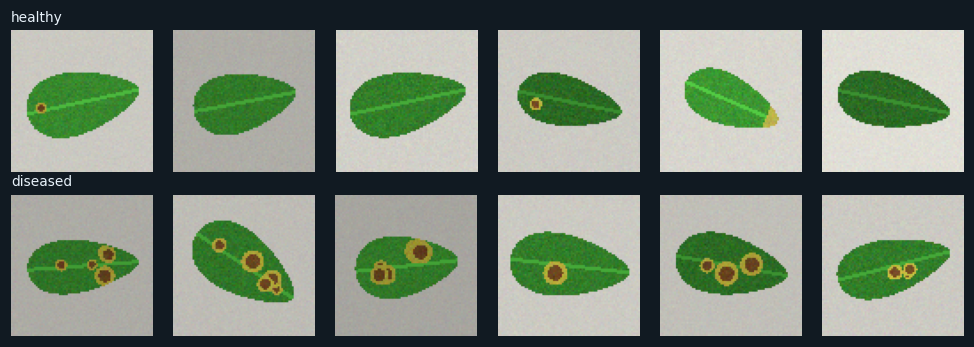
Healthy leaves on top, diseased leaves below, read from their folders and shown with plt.imshow().
Diseased leaves have brown spots with yellow rings. Some have many; some have only one or two small ones. Look at the healthy row too: one or two have a small spot or a yellow tip. The model has to learn how much brown and yellow is normal.
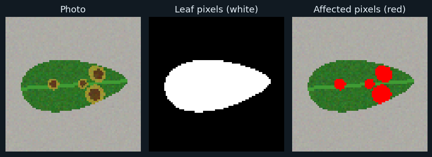
Left: the photo. Middle: the pixels counted as leaf, in white. Right: the leaf pixels counted as affected, painted red.
This is the whole idea of the project in one picture. The program cannot "see" a disease. What it can do is test every pixel with two simple rules: is it leaf, and is it brown or yellow instead of green? Counting the red pixels and dividing by the white ones gives the share of the leaf affected.
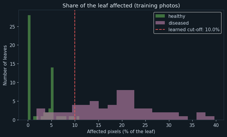
How many training leaves had each percentage of affected pixels, for healthy and diseased leaves. The dashed line is the cut-off the computer learned.
Healthy leaves bunch up near 0%, with a few up to about 11% because of blemishes and yellow tips. Diseased leaves spread from a few percent to over 40%. The two overlap on the left, where diseased leaves are at an early stage. The computer placed its cut-off at 10.0 % of the leaf affected, the point with the fewest mistakes.
📘 Revise: Stage 3 — Data Exploration
5Stage 4 — Modelling
Where this model sits in the family of AI models:
The answer is healthy or diseased, so this is classification. The training photos come from labelled folders, so it is supervised learning. The input is images, so it is Computer Vision.
How the model works
Each photo has been reduced to one feature: the percentage of the leaf that is affected. The photos are split into 120 for training and 30 for testing.
The model is a single cut-off: "diseased if the affected share is at least this much". The computer learns it by trying every cut-off from 0% to 40% in steps of 0.5%, counting the mistakes each would make on the training photos, and keeping the one with the fewest. It chose 10.0 % of the leaf affected, making 10 of 120 mistakes.
The severity levels used in deployment — mild below 15%, moderate below 30%, severe above — are rules written by a person, not learned. Grading disease by the share of leaf area affected is how plant scientists do it by eye, too.
📘 Revise: Stage 4 — Modelling
6Stage 5 — Evaluation
On 30 testing photos the accuracy was 90.0 %, with precision 100.0 % and recall 78.6 %.
The missed leaves are listed in the output, and they share one thing: each had less than 10% of its area affected. They are diseased leaves at the earliest stage — the very ones a farmer most needs to catch.
This is a trade-off worth thinking about. The cut-off was chosen to make the fewest mistakes overall, treating a false alarm and a miss as equally bad. For a farmer they are not equal: a false alarm costs a closer look; a miss lets a disease spread. A farmer's version should lower the cut-off a little — accepting a few false alarms to catch more early disease.
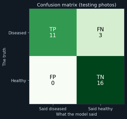
Diseased is the positive class. TP: diseased and caught. FN: diseased but called healthy. FP: healthy but called diseased. TN: healthy and called healthy.
On the testing photos the counts are 11 3 0 16 (TP, FN, FP, TN). No healthy leaf was called diseased, but some diseased leaves were missed.
📘 Revise: The Confusion Matrix
7Stage 6 — Deployment
The program checks four new leaves and prints, for each, the percentage affected and a severity: healthy, mild, moderate or severe. For any diseased leaf it gives the same advice: remove affected leaves, and show the photo to the nearest Krishi Vigyan Kendra before spraying anything.
As an app, the farmer would photograph a leaf on paper, and see the result and the affected area marked in red, exactly as in chart 2.
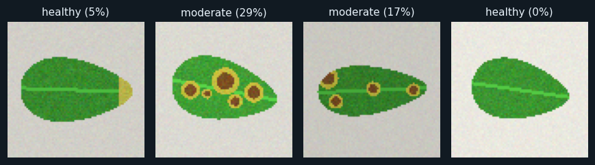
The four new leaves, each with its severity and the percentage affected.
Two are healthy and two diseased, and the model gets all four right. Beyond yes or no, it reports how much of each diseased leaf is affected — which tells a farmer how urgently to act.
📘 Revise: Stage 6 — Deployment
8Ethical concerns
An AI project is not finished when the model works. The curriculum asks three questions of every model — is it fair (bias), can it explain itself (transparency), and who answers for its mistakes (accountability). For this project:
The program says how much of a leaf is affected, not which disease it is or which chemical to use. Wrong spraying advice could waste a farmer's money and harm the soil and water, so that decision is left to an expert.
The model has learned one kind of leaf with one kind of spot. A different crop, or a disease that shows as black patches or white powder, may not be caught at all. It must be tested on the crop where it is used.
The model can show its working: the red pixels in chart 2 are exactly what it counted. A farmer can see why a leaf was called diseased.
📘 Revise: Bias, Transparency, Accountability
9Source code
The whole program — it is also in the downloads at the top of this page — in Python with pandas, NumPy and matplotlib — the three libraries of Unit 7. It is laid out as the six stages of the AI Project Cycle, one after another. Every chart on this page was drawn by it, and every number came out of running it.
# ---------------------------------------------------------------------------
# leaf_disease.py
#
# AI project on Computer Vision: spotting a diseased crop leaf from a photo,
# and saying how much of the leaf is affected.
#
# CBSE Class X, Artificial Intelligence (417), Part C project work.
# SDG 2 (Zero Hunger) and SDG 12 (Responsible Consumption and Production).
#
# The leaf is photographed on a plain sheet of paper. The program then:
#   1. finds which pixels are leaf and which are paper (segmentation),
#   2. counts how many leaf pixels are brown or yellow instead of green,
#   3. turns that into one FEATURE: the percentage of the leaf affected, and
#   4. learns, from the training photos, the cut-off percentage that best
#      separates healthy leaves from diseased ones.
#
# Libraries: numpy (pixel arithmetic), matplotlib (reading and showing
# images, and the charts), pandas (the table of features), os (folders).
# ---------------------------------------------------------------------------

# %% Stage 1 - Problem scoping
print("=" * 60)
print("IS THIS LEAF DISEASED?")
print("=" * 60)
print("Who   : farmers, especially those far from an expert")
print("What  : leaf disease noticed late spreads through the field")
print("Where : vegetable and crop fields, in the growing season")
print("Why   : early action saves the harvest and avoids extra spraying")
print()

# %% Stage 2 - Data acquisition
import os
import numpy as np
import pandas as pd
import matplotlib.pyplot as plt

pd.set_option("display.width", 120)

classes = ["healthy", "diseased"]
paths = []
labels = []
for c in classes:
    for name in sorted(os.listdir(os.path.join("images", c))):
        paths.append(os.path.join("images", c, name))
        labels.append(c)

print("--- Stage 2: Data acquisition ---")
print("Healthy leaves  :", labels.count("healthy"))
print("Diseased leaves :", labels.count("diseased"))
print("Total photos    :", len(paths))
print("Size of a photo :", plt.imread(paths[0]).shape)
print()

healthy_paths = []
diseased_paths = []
for i in range(len(paths)):
    if labels[i] == "healthy":
        healthy_paths.append(paths[i])
    else:
        diseased_paths.append(paths[i])

# Chart 1: six leaves of each kind.
plt.figure(figsize=(9, 3.2))
for i in range(6):
    plt.subplot(2, 6, i + 1)
    plt.imshow(plt.imread(healthy_paths[i * len(healthy_paths) // 6]))
    plt.axis("off")
    if i == 0:
        plt.title("healthy", fontsize=9, loc="left")
    plt.subplot(2, 6, i + 7)
    plt.imshow(plt.imread(diseased_paths[i * len(diseased_paths) // 6]))
    plt.axis("off")
    if i == 0:
        plt.title("diseased", fontsize=9, loc="left")
plt.tight_layout()
plt.savefig("chart1_sample_leaves.png")
plt.close()

# %% Stage 3 - Data exploration
print("--- Stage 3: Data exploration ---")

# Feature extraction, done the same way for every photo:
#   - Paper is grey: its red, green and blue are almost equal. A pixel whose
#     largest and smallest colour differ by more than 35 is leaf.
#   - Healthy leaf is green: much more green than red. A leaf pixel whose
#     red is at least 0.75 of its green is brown or yellow - affected.
rows = []
for i in range(len(paths)):
    img = plt.imread(paths[i])[:, :, :3].astype(float) * 255
    spread = img.max(axis=2) - img.min(axis=2)
    leaf = spread > 35
    affected = leaf & (img[:, :, 0] >= 0.75 * img[:, :, 1])
    percent = affected.sum() / leaf.sum() * 100
    rows.append([paths[i], labels[i], leaf.sum(), affected.sum(), round(percent, 1)])

data = pd.DataFrame(rows, columns=["photo", "label", "leaf_pixels", "affected_pixels", "affected_pct"])
print("Average of each kind:")
print(data.groupby("label")[["leaf_pixels", "affected_pixels", "affected_pct"]].mean().round(1))
print()
print("Healthy leaves  - most affected :", data[data["label"] == "healthy"]["affected_pct"].max(), "%")
print("Diseased leaves - least affected:", data[data["label"] == "diseased"]["affected_pct"].min(), "%")
print()

# Chart 2: what the program sees on one diseased leaf.
example = plt.imread(diseased_paths[0])[:, :, :3]
img = example.astype(float) * 255
leaf = (img.max(axis=2) - img.min(axis=2)) > 35
affected = leaf & (img[:, :, 0] >= 0.75 * img[:, :, 1])
marked = example.copy()
marked[affected] = [1.0, 0.0, 0.0]
plt.figure(figsize=(8, 3))
plt.subplot(1, 3, 1)
plt.imshow(example)
plt.title("Photo")
plt.axis("off")
plt.subplot(1, 3, 2)
plt.imshow(leaf, cmap="gray")
plt.title("Leaf pixels (white)")
plt.axis("off")
plt.subplot(1, 3, 3)
plt.imshow(marked)
plt.title("Affected pixels (red)")
plt.axis("off")
plt.tight_layout()
plt.savefig("chart2_pixel_masks.png")
plt.close()

# %% Stage 4 - Modelling
print("--- Stage 4: Modelling ---")
data = data.sample(frac=1, random_state=4)
cut = int(len(data) * 0.8)
train = data[:cut]
test = data[cut:]
print("Training photos :", len(train))
print("Testing photos  :", len(test))

# Learn the cut-off: try every value from 0% to 40% in steps of 0.5, count
# the training mistakes of "diseased if affected_pct is at least this", and
# keep the cut-off with the fewest.
truth = train["label"] == "diseased"
best_cutoff = 0
best_mistakes = len(train) + 1
cutoffs = np.arange(0, 40.5, 0.5)
for c in cutoffs:
    mistakes = ((train["affected_pct"] >= c) != truth).sum()
    if mistakes < best_mistakes:
        best_mistakes = mistakes
        best_cutoff = c
print("Learned cut-off            :", best_cutoff, "% of the leaf affected")
print("Mistakes on training data  :", best_mistakes, "of", len(train))
print()

# Chart 3: the feature for both kinds, with the learned cut-off.
plt.figure(figsize=(7, 4.3))
plt.hist(train[train["label"] == "healthy"]["affected_pct"], bins=20, alpha=0.65, color="#59a14f", label="healthy")
plt.hist(train[train["label"] == "diseased"]["affected_pct"], bins=20, alpha=0.65, color="#b07aa1", label="diseased")
plt.axvline(best_cutoff, color="#e15759", linestyle="--", label="learned cut-off: " + str(best_cutoff) + "%")
plt.title("Share of the leaf affected (training photos)")
plt.xlabel("Affected pixels (% of the leaf)")
plt.ylabel("Number of leaves")
plt.legend()
plt.tight_layout()
plt.savefig("chart3_affected_share.png")
plt.close()

# %% Stage 5 - Evaluation
print("--- Stage 5: Evaluation ---")
tp = fn = fp = tn = 0
wrong = []
for i in range(len(test)):
    row = test.iloc[i]
    said_diseased = row["affected_pct"] >= best_cutoff
    if row["label"] == "diseased" and said_diseased:
        tp = tp + 1
    elif row["label"] == "diseased":
        fn = fn + 1
        wrong.append(i)
    elif said_diseased:
        fp = fp + 1
        wrong.append(i)
    else:
        tn = tn + 1
accuracy = (tp + tn) / len(test) * 100
precision = 0
if tp + fp > 0:
    precision = tp / (tp + fp) * 100
recall = 0
if tp + fn > 0:
    recall = tp / (tp + fn) * 100
f1 = 0
if precision + recall > 0:
    f1 = 2 * precision * recall / (precision + recall)
print("TP, FN, FP, TN :", tp, fn, fp, tn)
print("Accuracy       :", round(accuracy, 1), "%")
print("Precision      :", round(precision, 1), "%")
print("Recall         :", round(recall, 1), "%")
print("F1 score       :", round(f1, 1), "%")
print("Photos wrong   :", len(wrong))
for i in wrong:
    row = test.iloc[i]
    print("  " + os.path.basename(row["photo"]), "really", row["label"], "-", row["affected_pct"], "% affected")
print()

# Chart 4: confusion matrix.
grid = [[tp, fn], [fp, tn]]
plt.figure(figsize=(5, 4.3))
plt.imshow(grid, cmap="Greens")
names = [["TP", "FN"], ["FP", "TN"]]
for r in range(2):
    for c in range(2):
        if grid[r][c] > max(max(grid)) / 2:
            ink = "white"
        else:
            ink = "black"
        plt.text(c, r, names[r][c] + "\n" + str(grid[r][c]), ha="center", va="center", fontsize=14, color=ink)
plt.xticks([0, 1], ["Said diseased", "Said healthy"])
plt.yticks([0, 1], ["Diseased", "Healthy"])
plt.xlabel("What the model said")
plt.ylabel("The truth")
plt.title("Confusion matrix (testing photos)")
plt.tight_layout()
plt.savefig("chart4_matrix.png")
plt.close()

# %% Stage 6 - Deployment
print("--- Stage 6: Deployment ---")
new_names = sorted(os.listdir("new_photos"))
plt.figure(figsize=(8, 2.8))
for i in range(len(new_names)):
    photo = plt.imread(os.path.join("new_photos", new_names[i]))[:, :, :3]
    img = photo.astype(float) * 255
    leaf = (img.max(axis=2) - img.min(axis=2)) > 35
    affected = leaf & (img[:, :, 0] >= 0.75 * img[:, :, 1])
    percent = affected.sum() / leaf.sum() * 100
    if percent < best_cutoff:
        verdict = "healthy"
    elif percent < 15:
        verdict = "mild"
    elif percent < 30:
        verdict = "moderate"
    else:
        verdict = "severe"
    print(new_names[i], "->", round(percent, 1), "% affected ->", verdict.upper())
    plt.subplot(1, len(new_names), i + 1)
    plt.imshow(photo)
    plt.title(verdict + " (" + str(round(percent)) + "%)", fontsize=10)
    plt.axis("off")
plt.tight_layout()
plt.savefig("chart5_new_leaves.png")
plt.close()
print("Mild, moderate or severe: remove affected leaves and show the photo to")
print("the nearest Krishi Vigyan Kendra before spraying anything.")
The library calls it is built from
| Call | Where | What it does |
|---|---|---|
os.listdir() | Stage 2 | Lists the photos in each folder |
plt.imread() / plt.imshow() | Stages 2, 3, 6 | Reads and shows the photos |
img.max(axis=2) - img.min(axis=2) | Stage 3 | How coloured each pixel is — near 0 for grey paper |
spread > 35 | Stage 3 | Marks the leaf pixels (segmentation) |
img[:, :, 0] >= 0.75 * img[:, :, 1] | Stage 3 | Marks pixels where red is close to green: brown or yellow |
mask.sum() | Stage 3 | Counts the pixels in a mask |
marked[affected] = [1, 0, 0] | Stage 3 | Paints the affected pixels red, for chart 2 |
np.arange(0, 40.5, 0.5) | Stage 4 | Every cut-off to try |
((pct >= c) != truth).sum() | Stage 4 | The mistakes one cut-off makes |
10Sample output
A real run, exactly as it appeared. Nothing below was typed by hand.
============================================================
IS THIS LEAF DISEASED?
============================================================
Who   : farmers, especially those far from an expert
What  : leaf disease noticed late spreads through the field
Where : vegetable and crop fields, in the growing season
Why   : early action saves the harvest and avoids extra spraying

--- Stage 2: Data acquisition ---
Healthy leaves  : 75
Diseased leaves : 75
Total photos    : 150
Size of a photo : (80, 80, 3)

--- Stage 3: Data exploration ---
Average of each kind:
          leaf_pixels  affected_pixels  affected_pct
label
diseased       1531.8            272.1          17.8
healthy        1515.9             41.1           2.7

Healthy leaves  - most affected : 10.9 %
Diseased leaves - least affected: 1.8 %

--- Stage 4: Modelling ---
Training photos : 120
Testing photos  : 30
Learned cut-off            : 10.0 % of the leaf affected
Mistakes on training data  : 10 of 120

--- Stage 5: Evaluation ---
TP, FN, FP, TN : 11 3 0 16
Accuracy       : 90.0 %
Precision      : 100.0 %
Recall         : 78.6 %
F1 score       : 88.0 %
Photos wrong   : 3
  diseased_020.png really diseased - 4.4 % affected
  diseased_035.png really diseased - 8.3 % affected
  diseased_063.png really diseased - 7.4 % affected

--- Stage 6: Deployment ---
leaf_1.png -> 5.2 % affected -> HEALTHY
leaf_2.png -> 28.8 % affected -> MODERATE
leaf_3.png -> 17.1 % affected -> MODERATE
leaf_4.png -> 0.0 % affected -> HEALTHY
Mild, moderate or severe: remove affected leaves and show the photo to
the nearest Krishi Vigyan Kendra before spraying anything.11The same project without code
Teachable Machine learns from the photos directly, without any rules about colour; comparing it with this program shows what hand-made features can and cannot do. The tool is Teachable Machine (or Orange with the Image Analytics add-on).
Choose an Image Project, standard image model.
Name them healthy and diseased, and upload the photos from each folder.
Train, then open Advanced to see the accuracy per class.
Test it with the leaves in new_photos.
Load the images folder and turn the photos into features.
Train and test a model on the embeddings.
Look at the misclassified leaves — are they the early-stage ones here, too?
📘 Revise: No-Code AI, and Orange
12Testing
Every case below was actually run, and the result is what came back. Each one gives the whole program a small input of its own.
| Test case | Expected | Actual | Result |
|---|---|---|---|
| All 150 photos are read | Total photos : 150 | Total photos : 150 | Pass |
| The computer learns the cut-off from the training photos | Learned cut-off : 10.0 % of the leaf affected | Learned cut-off : 10.0 % of the leaf affected | Pass |
| No healthy leaf is called diseased | Precision : 100.0 % | Precision : 100.0 % | Pass |
| The early-stage leaves are the ones it misses | Photos wrong : 3 | Photos wrong : 3 | Pass |
| Clean green leaves against 30% brown ones: no mistakes | Accuracy : 100.0 % | Accuracy : 100.0 % | Pass |
| A fully green new leaf: 0% affected | leaf_1.png -> 0.0 % affected -> HEALTHY | leaf_1.png -> 0.0 % affected -> HEALTHY | Pass |
| 4 brown rows of 40 is exactly 10% affected: mild (under 15%) | leaf_2.png -> 10.0 % affected -> MILD | leaf_2.png -> 10.0 % affected -> MILD | Pass |
| 25% affected is moderate | leaf_3.png -> 25.0 % affected -> MODERATE | leaf_3.png -> 25.0 % affected -> MODERATE | Pass |
| 50% affected is severe | leaf_4.png -> 50.0 % affected -> SEVERE | leaf_4.png -> 50.0 % affected -> SEVERE | Pass |
13Results, limits and what next
- Leaf and paper separate cleanly by how coloured a pixel is; brown and yellow separate from green by comparing red with green.
- Healthy leaves have up to about 11% of their area off-colour, from blemishes and ageing tips.
- The computer learned a cut-off of 10.0 % of the leaf affected.
- On unseen photos it reached an accuracy of 90.0 %, with no false alarms.
- Every leaf it missed was at the earliest stage, with less than 10% affected.
What this model cannot do
- Pictures drawn by a program, simpler than real leaves
- It needs a plain paper background; in the field, soil and other leaves would confuse it
- It measures how much is affected, not which disease it is
- Early-stage disease is the hardest to catch, and that is when it matters most
What to add next
This is where you make the project your own. Take one of these, or an idea of yours:
- Lower the cut-off and see how many more early cases are caught, and at what cost in false alarms
- Photograph real leaves from a school garden and retrain
- Add a second feature, such as the number of separate spots
- Compare with a Teachable Machine model trained on the same photos
What you may have to learn on your own
- How to test every pixel in an image with a rule, using numpy masks
- Segmentation: separating an object from its background
- Why a percentage is fairer than a count
- How a cut-off is learned, and why the best cut-off depends on which mistake is worse
14Conclusion
The project showed that a phone photo of a leaf on paper can be turned into a clear, honest number: the share of the leaf affected. With a cut-off learned from the training photos, the model was right 90.0 % of the time on photos it had never seen, and never raised a false alarm.
The mistakes were all early-stage leaves — the cases a farmer most needs. That is not a reason to give up on the model; it is the reason to choose the cut-off for the farmer's needs rather than for the fewest mistakes overall.
Because the program shows exactly which pixels it counted, its decisions can be checked by anyone looking at the red marks — which matters when the advice affects a family's harvest.
15Questions for the viva
The project carries a viva voce of its own, worth 5 marks. These are the questions it is most likely to ask about this project. Try answering each one aloud before opening it.
▸What feature did your model use?
The percentage of the leaf that is brown or yellow instead of green.
▸How did you find the leaf pixels?
Paper is grey, so its red, green and blue values are almost equal. A pixel whose largest and smallest colour values differ by more than 35 is leaf.
▸How did you decide a pixel was diseased?
Healthy leaf has much more green than red. If a leaf pixel's red is at least 0.75 of its green, it is brown or yellow.
▸Why use a percentage instead of a count?
So a big leaf does not look more diseased than a small one just because it has more pixels.
▸Which leaves did your model miss?
Diseased leaves at an early stage, with less than 10% of the leaf affected.
▸Should you use the cut-off with the fewest mistakes?
Not necessarily. For a farmer, missing a disease is worse than a false alarm, so a slightly lower cut-off would be better.
▸Which SDGs does it relate to?
SDG 2, Zero Hunger, and SDG 12, Responsible Consumption and Production.
16References
- Food and Agriculture Organization of the United Nations, plant health and crop losses — https://www.fao.org/plant-health/
- Krishi Vigyan Kendra Knowledge Network, ICAR — https://kvk.icar.gov.in/
- Hughes, D. P. and Salathé, M. (2015). An open access repository of images on plant health (PlantVillage). arXiv:1511.08060.
- Teachable Machine — https://teachablemachine.withgoogle.com/
- CBSE, Artificial Intelligence (Subject Code 417), Class X curriculum, 2026-27 — Part C, Practical and Project Work
- CBSE, Artificial Intelligence Facilitator Handbook, Class X
- pandas — https://pandas.pydata.org/docs/; NumPy — https://numpy.org/doc/; Matplotlib — https://matplotlib.org/stable/
- LambdaLab — https://www.lambdalab.in