Finding Cracks with Convolution
An edge-detecting kernel slides over a photo of a wall, and the cracks light up while the harmless stains do not — the convolution operator from Unit 5, doing a real job.
1Introduction
Every building cracks a little as it ages, and most cracks are harmless — but some are the first sign of a serious problem. Inspectors photograph walls and then go through the photos looking for cracks.
There is a catch. Walls also have damp stains, dirty patches and shadows. They are dark too, and a quick look — or a simple computer rule like "look for dark patches" — mistakes them for cracks.
This project uses the convolution operator from Unit 5 to tell the two apart. A crack is thin and sharp; a stain is wide and soft. An edge-detecting kernel reacts to exactly that difference.
Industry, Innovation and Infrastructure
Sustainable Cities and Communities
SDG 9 asks for infrastructure that is reliable and resilient, and SDG 11 for cities that are safe. Buildings, bridges and flyovers develop cracks as they age. Found early, a crack is a cheap repair; found late, it can mean a collapse. Inspecting every wall by eye is slow, so a tool that flags cracks in photos helps engineers check more structures, more often.
The curriculum asks that the project be related to the Sustainable Development Goals. That link is the reason the problem is worth solving, so it belongs at the very start of the report, not tacked on at the end.
2Stage 1 — Problem Scoping
Problem scoping means understanding the problem properly before building anything. The tool for it is the 4Ws Problem Canvas: who has the problem, what the problem is, where it happens, and why solving it matters.
- Engineers and inspectors of buildings and bridges
- People who use those buildings every day
- Cracks can be missed in hundreds of inspection photos
- Harmless stains are mistaken for cracks, wasting inspectors' time
- Old buildings, flyovers, bridges and school walls
- After the monsoon, when damp stains are everywhere
- Cracks found early can be repaired before they are dangerous
- Inspectors spend their time on real problems
The problem statement
The four answers are then joined into one sentence, using the curriculum's problem statement template:
Engineers and inspectors who check buildings, bridges and school walls, and a school's maintenance staff after the monsoon.
How it is done today
An experienced engineer is the best judge, but checking every wall of every building often is slow and expensive.
Faster than visiting every wall, but going through hundreds of photos is tiring, and tired eyes miss things.
The obvious automatic method — flag anything dark. This project tests it and shows why it is not good enough.
Objectives
- To read wall photos and turn them into grayscale
- To apply an edge-detecting convolution kernel to every photo
- To measure two features: how much of the wall is dark, and how much the kernel lights up
- To let the computer learn a cut-off for each feature from the training photos
- To compare the two models on unseen photos and explain the difference
- To flag new wall photos for an engineer to check
📘 Revise: Stage 1 — Problem Scoping
3Stage 2 — Data Acquisition
The data is a folder of wall photos sorted into images/cracked/ and images/sound/ (sound means no crack).
There are 140 photos, each 64 × 64 pixels. Many of the sound walls have a damp stain or dirty patch on purpose, because that is what makes the problem hard. Four more photos in new_photos/ are used for deployment.
The walls were drawn by a program. For your own project, photograph walls around your school (with permission) — cracks and stains both — or use a public concrete-crack image dataset and credit it.
Features and label
The features are what the model is given. The label is the answer it has to learn to give.
| Column | Type | What it holds | Role |
|---|---|---|---|
dark_pct | decimal | Share of pixels much darker than the wall's usual shade (more than 25 below its median) | feature (model A) |
edge_pct | decimal | Share of pixels the edge kernel lights up (output above 60) | feature (model B) |
label | text | cracked or sound — the folder it came from | label |
photo | file | The wall photo, turned into a 64 × 64 grayscale grid | not used |
Inside the images/ folder
Wall photos in a cracked folder and a sound folder. Many sound walls carry a stain. There are 140 images, 731.2 KB in all, one folder per class — the same layout Teachable Machine and Orange expect:
The images come with the project download.
Inside the new_photos/ folder
Four new wall photos, used in the deployment stage. There are 4 images, 20.8 KB in all.
The images come with the project download.
📘 Revise: Stage 2 — Data Acquisition
4Stage 3 — Data Exploration
Data exploration means getting to know the data before trusting it: fixing what is wrong with it, then drawing it to see the patterns. The charts here are what decide what the model should be.
What was wrong with the data
A crack is about light and dark, not colour, so each photo is turned into grayscale by averaging its red, green and blue values. One grid of numbers is simpler than three.
Some walls are light, some darker. So "dark" is measured against each wall's own usual shade (its median) rather than against a fixed number.
Kept on purpose. A dataset of clean walls would make the problem look easy and the model would fail on real walls.
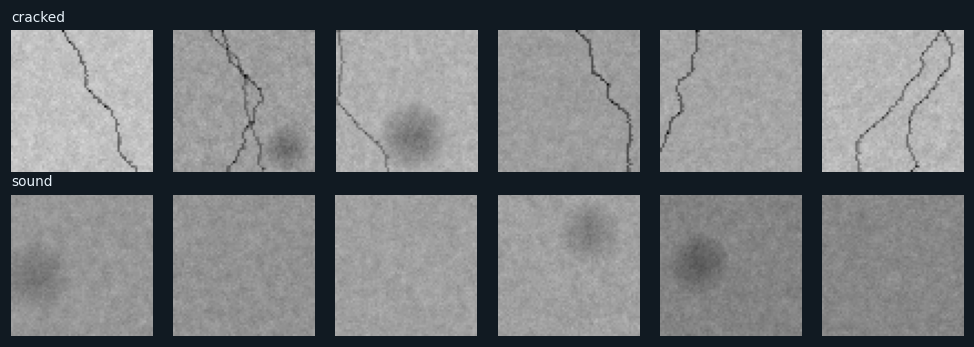
Cracked walls on top, sound walls below.
The cracks are thin dark lines that wander across the wall. Look at the sound walls: several have a dark, soft stain. Both are dark. What differs is the shape — thin and sharp, or wide and soft.
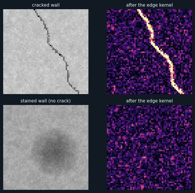
Left: a cracked wall and a stained wall in grayscale. Right: the same walls after the edge kernel has been slid over them. Bright means the kernel's output was large.
This is the whole project in one picture. On the cracked wall the crack lights up as a bright line. On the stained wall the stain all but disappears. The kernel weighs the centre pixel +4 and its four neighbours −1 each, so on a smooth patch — even a dark one — they cancel out to almost nothing. Only a sharp change, like a thin crack, survives.
The output is 62 × 62, two pixels smaller each way than the photo, because the kernel cannot be centred on the edge pixels — exactly as Unit 5 describes.
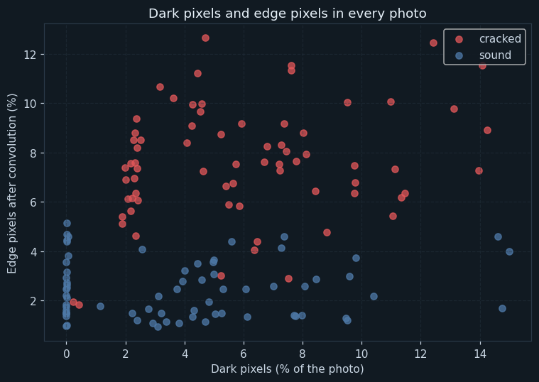
Each dot is one photo: its share of dark pixels across, its share of edge pixels up.
Along the bottom axis the two kinds are mixed together — stained walls are as dark as cracked ones. Up the side they separate: cracked walls have many more edge pixels. So the convolution feature should make the better model.
📘 Revise: Stage 3 — Data Exploration
5Stage 4 — Modelling
Where this model sits in the family of AI models:
The answer is cracked or sound, so this is classification. The photos are labelled by folder, so it is supervised learning, in the Computer Vision domain.
How the model works
Every photo is turned into grayscale, then the edge kernel is slid over it. At each position the 9 pixels under the kernel are multiplied by the 9 kernel numbers and added up — that is convolution. The program does this for every position at once by adding up nine shifted copies of the image, which gives exactly the same answer as sliding the kernel one step at a time.
The photos are split into 112 for training and 28 for testing. Each of the two models has the form "cracked if this feature is at least this cut-off". The computer learns each cut-off by trying every value the feature takes in the training photos and keeping the one with the fewest mistakes.
This is the idea behind the Convolutional Neural Networks of Unit 5, done by hand. Here a person chose the kernel. A CNN starts with random kernels and learns, from thousands of photos, which ones bring out the features that matter.
📘 Revise: Stage 4 — Modelling
6Stage 5 — Evaluation
Both models were tested on the same 28 photos. The dark-pixel model scored an accuracy of 64.3 %, with precision 50.0 %: it flagged stained walls as cracked. The convolution model scored 96.4 %, with precision 90.9 %.
Both had a recall of 100% — neither missed a crack. For safety that is the most important number, because a missed crack could be dangerous. But a model with low precision is not useful either: an inspector sent to every stained wall soon stops trusting it. The convolution model keeps the recall and fixes the precision.
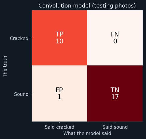
Cracked is the positive class. TP: cracked and flagged. FN: cracked but missed. FP: sound but flagged. TN: sound and passed.
On the testing photos the counts are 10 0 1 17 (TP, FN, FP, TN). No crack was missed.
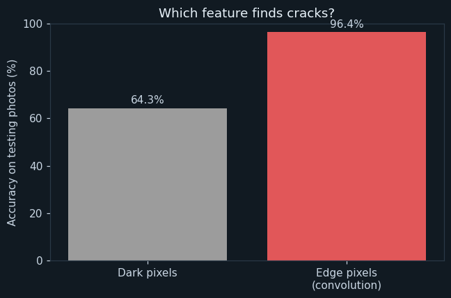
The accuracy of each model on the same testing photos.
The dark-pixel model reached only 64.3 %; the convolution model reached 96.4 %. Same photos, same way of learning a cut-off — the only difference is the feature. Choosing the right feature mattered more than anything else in the project.
📘 Revise: The Confusion Matrix
7Stage 6 — Deployment
The program checks four new walls and prints, for each, the share of edge pixels and a verdict: "CRACK — send an engineer" or "no crack found".
In real use, an inspector or a drone would photograph every wall, and the program would sort the photos so the engineer sees the flagged ones first. The engineer still decides whether a crack is serious.
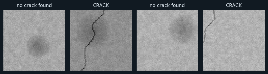
Four new wall photos, each with the convolution model's verdict.
The two cracked walls are flagged and the two sound walls are passed.
📘 Revise: Stage 6 — Deployment
8Ethical concerns
An AI project is not finished when the model works. The curriculum asks three questions of every model — is it fair (bias), can it explain itself (transparency), and who answers for its mistakes (accountability). For this project:
A missed crack could put lives at risk. The model can sort photos, but a qualified engineer must make every decision about whether a building is safe.
The model learned one kind of wall. Brick, tiles, painted surfaces with patterns, or hairline cracks thinner than a pixel may fool it. It must be tested on the walls it will really check.
The edge map in chart 2 shows exactly what the model is responding to. An engineer can look at it and see why a photo was flagged.
📘 Revise: Bias, Transparency, Accountability
9Source code
The whole program — it is also in the downloads at the top of this page — in Python with pandas, NumPy and matplotlib — the three libraries of Unit 7. It is laid out as the six stages of the AI Project Cycle, one after another. Every chart on this page was drawn by it, and every number came out of running it.
# ---------------------------------------------------------------------------
# wall_cracks.py
#
# AI project on Computer Vision: finding cracks in photos of concrete walls,
# using the CONVOLUTION operator from Unit 5.
#
# CBSE Class X, Artificial Intelligence (417), Part C project work.
# SDG 9 (Industry, Innovation and Infrastructure) and SDG 11 (Sustainable
# Cities and Communities).
#
# A crack is dark - but so is a damp stain, which is harmless. The
# difference is that a crack is THIN and SHARP, while a stain is wide and
# soft. A convolution kernel that detects edges reacts strongly to thin
# sharp lines and hardly at all to soft patches. The project compares:
#   - Model A: uses only how much of the wall is DARK
#   - Model B: uses how much of the wall the edge kernel LIGHTS UP
# Each model learns its own cut-off from the training photos.
#
# Libraries: numpy (the convolution), matplotlib (images and charts),
# pandas (the table of features), os (the folders).
# ---------------------------------------------------------------------------

# %% Stage 1 - Problem scoping
print("=" * 60)
print("FINDING CRACKS WITH CONVOLUTION")
print("=" * 60)
print("Who   : engineers who inspect buildings, bridges and school walls")
print("What  : cracks are missed, or stains are mistaken for cracks")
print("Where : old buildings, flyovers and walls after heavy rain")
print("Why   : a crack found early can be repaired before it is dangerous")
print()

# %% Stage 2 - Data acquisition
import os
import numpy as np
import pandas as pd
import matplotlib.pyplot as plt

pd.set_option("display.width", 120)

classes = ["cracked", "sound"]
paths = []
labels = []
for c in classes:
    for name in sorted(os.listdir(os.path.join("images", c))):
        paths.append(os.path.join("images", c, name))
        labels.append(c)

print("--- Stage 2: Data acquisition ---")
print("Cracked walls :", labels.count("cracked"))
print("Sound walls   :", labels.count("sound"))
print("Total photos  :", len(paths))
print()

cracked_paths = []
sound_paths = []
for i in range(len(paths)):
    if labels[i] == "cracked":
        cracked_paths.append(paths[i])
    else:
        sound_paths.append(paths[i])

# Chart 1: six walls of each kind.
plt.figure(figsize=(9, 3.2))
for i in range(6):
    plt.subplot(2, 6, i + 1)
    plt.imshow(plt.imread(cracked_paths[i * len(cracked_paths) // 6]))
    plt.axis("off")
    if i == 0:
        plt.title("cracked", fontsize=9, loc="left")
    plt.subplot(2, 6, i + 7)
    plt.imshow(plt.imread(sound_paths[i * len(sound_paths) // 6]))
    plt.axis("off")
    if i == 0:
        plt.title("sound", fontsize=9, loc="left")
plt.tight_layout()
plt.savefig("chart1_sample_walls.png")
plt.close()

# %% Stage 3 - Data exploration
print("--- Stage 3: Data exploration ---")

# The edge-detecting kernel. The centre pixel is weighed +4 and its four
# neighbours -1 each. On a flat patch they cancel out to about 0; on a thin
# line, where the centre is very different from its neighbours, the result
# is large.
kernel = np.array([[0, -1, 0],
                   [-1, 4, -1],
                   [0, -1, 0]])
print("The kernel:")
print(kernel)
print()

# Convolution: slide the 3 x 3 kernel over every position in the image,
# multiply each of the 9 pixels under it by the matching kernel number, and
# add the 9 results up. Done here for all positions at once: for each of the
# 9 kernel cells, take the part of the image under it and add it in.
# The output is 2 pixels smaller each way, because the kernel cannot be
# centred on the edge pixels.
rows = []
for i in range(len(paths)):
    grey = plt.imread(paths[i])[:, :, :3].astype(float).mean(axis=2) * 255   # grayscale, 0-255
    h, w = grey.shape
    edges = np.zeros((h - 2, w - 2))
    for dy in range(3):
        for dx in range(3):
            edges = edges + kernel[dy, dx] * grey[dy:dy + h - 2, dx:dx + w - 2]
    dark_pct = (grey < np.median(grey) - 25).mean() * 100     # much darker than the wall
    edge_pct = (np.abs(edges) > 60).mean() * 100              # lit up by the kernel
    rows.append([paths[i], labels[i], round(dark_pct, 2), round(edge_pct, 2)])

data = pd.DataFrame(rows, columns=["photo", "label", "dark_pct", "edge_pct"])
print("Size of a photo            :", h, "x", w)
print("Size after the convolution :", h - 2, "x", w - 2)
print()
print("Average features of each kind:")
print(data.groupby("label")[["dark_pct", "edge_pct"]].mean().round(2))
print()

# Chart 2: what the kernel does to a cracked wall and to a stained one.
stained = None
for p in sound_paths:
    g = plt.imread(p)[:, :, :3].astype(float).mean(axis=2) * 255
    if (g < np.median(g) - 25).mean() > 0.05:
        stained = p
        break
plt.figure(figsize=(7, 6.2))
pair = [cracked_paths[0], stained]
titles = ["cracked wall", "stained wall (no crack)"]
for n in range(2):
    grey = plt.imread(pair[n])[:, :, :3].astype(float).mean(axis=2) * 255
    h, w = grey.shape
    edges = np.zeros((h - 2, w - 2))
    for dy in range(3):
        for dx in range(3):
            edges = edges + kernel[dy, dx] * grey[dy:dy + h - 2, dx:dx + w - 2]
    plt.subplot(2, 2, n * 2 + 1)
    plt.imshow(grey, cmap="gray", vmin=0, vmax=255)
    plt.title(titles[n], fontsize=10)
    plt.axis("off")
    plt.subplot(2, 2, n * 2 + 2)
    plt.imshow(np.abs(edges), cmap="magma", vmin=0, vmax=150)
    plt.title("after the edge kernel", fontsize=10)
    plt.axis("off")
plt.tight_layout()
plt.savefig("chart2_convolution.png")
plt.close()

# Chart 3: the two features, one dot per photo.
plt.figure(figsize=(7, 5))
dot = ["#e15759", "#4e79a7"]
for k in range(2):
    part = data[data["label"] == classes[k]]
    plt.scatter(part["dark_pct"], part["edge_pct"], color=dot[k], label=classes[k], alpha=0.75)
plt.title("Dark pixels and edge pixels in every photo")
plt.xlabel("Dark pixels (% of the photo)")
plt.ylabel("Edge pixels after convolution (%)")
plt.legend()
plt.grid(True, linestyle="--", alpha=0.4)
plt.tight_layout()
plt.savefig("chart3_features.png")
plt.close()

# %% Stage 4 - Modelling
print("--- Stage 4: Modelling ---")
data = data.sample(frac=1, random_state=9)
cut = int(len(data) * 0.8)
train = data[:cut]
test = data[cut:]
print("Training photos :", len(train))
print("Testing photos  :", len(test))
print()

# Each model is "cracked if <feature> is at least <cut-off>". The cut-off is
# learned: try every value the feature takes in the training photos, and
# keep the one with the fewest training mistakes.
truth = train["label"] == "cracked"
learned = {}
for feature in ["dark_pct", "edge_pct"]:
    best = None
    for c in sorted(train[feature].unique()):
        mistakes = ((train[feature] >= c) != truth).sum()
        if best is None or mistakes < best[1]:
            best = [c, mistakes]
    learned[feature] = best[0]
    print("Model using", feature.ljust(9), ": cracked if", feature, ">=", best[0],
          " (" + str(best[1]), "training mistakes)")
print()

# %% Stage 5 - Evaluation
print("--- Stage 5: Evaluation ---")
results = {}
for feature in ["dark_pct", "edge_pct"]:
    tp = fn = fp = tn = 0
    for i in range(len(test)):
        row = test.iloc[i]
        said = row[feature] >= learned[feature]
        if row["label"] == "cracked" and said:
            tp = tp + 1
        elif row["label"] == "cracked":
            fn = fn + 1
        elif said:
            fp = fp + 1
        else:
            tn = tn + 1
    results[feature] = [tp, fn, fp, tn]
    accuracy = (tp + tn) / len(test) * 100
    recall = 0
    if tp + fn > 0:
        recall = tp / (tp + fn) * 100
    precision = 0
    if tp + fp > 0:
        precision = tp / (tp + fp) * 100
    print("Model using " + feature)
    print("  " + feature + " TP, FN, FP, TN :", tp, fn, fp, tn)
    print("  " + feature + " accuracy  :", round(accuracy, 1), "%")
    print("  " + feature + " precision :", round(precision, 1), "%")
    print("  " + feature + " recall    :", round(recall, 1), "%")
    print()

# Chart 4: confusion matrix of the convolution model.
tp, fn, fp, tn = results["edge_pct"]
grid = [[tp, fn], [fp, tn]]
plt.figure(figsize=(5, 4.3))
plt.imshow(grid, cmap="Reds")
names = [["TP", "FN"], ["FP", "TN"]]
for r in range(2):
    for c in range(2):
        if grid[r][c] > max(max(grid)) / 2:
            ink = "white"
        else:
            ink = "black"
        plt.text(c, r, names[r][c] + "\n" + str(grid[r][c]), ha="center", va="center", fontsize=14, color=ink)
plt.xticks([0, 1], ["Said cracked", "Said sound"])
plt.yticks([0, 1], ["Cracked", "Sound"])
plt.xlabel("What the model said")
plt.ylabel("The truth")
plt.title("Convolution model (testing photos)")
plt.tight_layout()
plt.savefig("chart4_matrix.png")
plt.close()

# Chart 5: the two models compared.
acc_dark = (results["dark_pct"][0] + results["dark_pct"][3]) / len(test) * 100
acc_edge = (results["edge_pct"][0] + results["edge_pct"][3]) / len(test) * 100
plt.figure(figsize=(6, 4))
plt.bar(["Dark pixels", "Edge pixels\n(convolution)"], [acc_dark, acc_edge], color=["#9c9c9c", "#e15759"])
plt.ylim(0, 100)
plt.ylabel("Accuracy on testing photos (%)")
plt.title("Which feature finds cracks?")
plt.text(0, acc_dark + 2, str(round(acc_dark, 1)) + "%", ha="center")
plt.text(1, acc_edge + 2, str(round(acc_edge, 1)) + "%", ha="center")
plt.tight_layout()
plt.savefig("chart5_models.png")
plt.close()

# %% Stage 6 - Deployment
print("--- Stage 6: Deployment ---")
new_names = sorted(os.listdir("new_photos"))
plt.figure(figsize=(8, 2.7))
for i in range(len(new_names)):
    grey = plt.imread(os.path.join("new_photos", new_names[i]))[:, :, :3].astype(float).mean(axis=2) * 255
    h, w = grey.shape
    edges = np.zeros((h - 2, w - 2))
    for dy in range(3):
        for dx in range(3):
            edges = edges + kernel[dy, dx] * grey[dy:dy + h - 2, dx:dx + w - 2]
    edge_pct = (np.abs(edges) > 60).mean() * 100
    if edge_pct >= learned["edge_pct"]:
        verdict = "CRACK - send an engineer"
    else:
        verdict = "no crack found"
    print(new_names[i], "-> edge pixels", round(edge_pct, 2), "% ->", verdict)
    plt.subplot(1, len(new_names), i + 1)
    plt.imshow(grey, cmap="gray", vmin=0, vmax=255)
    plt.title(verdict.split(" - ")[0], fontsize=10)
    plt.axis("off")
plt.tight_layout()
plt.savefig("chart6_new_walls.png")
plt.close()
The library calls it is built from
| Call | Where | What it does |
|---|---|---|
plt.imread() | Stages 2, 3, 6 | Reads a wall photo |
img.mean(axis=2) | Stage 3 | Turns a colour photo into grayscale |
np.array([[0,-1,0],[-1,4,-1],[0,-1,0]]) | Stage 3 | The edge-detecting kernel |
grey[dy:dy + h - 2, dx:dx + w - 2] | Stage 3 | The part of the image under one kernel cell |
edges = edges + kernel[dy, dx] * ... | Stage 3 | Multiplies and adds — the convolution |
np.abs(edges) > 60 | Stage 3 | Marks the pixels the kernel lit up |
np.median(grey) | Stage 3 | The wall's usual shade |
plt.imshow(..., cmap="magma") | Stage 3 | Shows the kernel's output as a heat map |
sorted(train[f].unique()) | Stage 4 | Every cut-off to try |
10Sample output
A real run, exactly as it appeared. Nothing below was typed by hand.
============================================================
FINDING CRACKS WITH CONVOLUTION
============================================================
Who   : engineers who inspect buildings, bridges and school walls
What  : cracks are missed, or stains are mistaken for cracks
Where : old buildings, flyovers and walls after heavy rain
Why   : a crack found early can be repaired before it is dangerous

--- Stage 2: Data acquisition ---
Cracked walls : 70
Sound walls   : 70
Total photos  : 140

--- Stage 3: Data exploration ---
The kernel:
[[ 0 -1  0]
 [-1  4 -1]
 [ 0 -1  0]]

Size of a photo            : 64 x 64
Size after the convolution : 62 x 62

Average features of each kind:
         dark_pct  edge_pct
label
cracked      5.99      7.58
sound        3.90      2.44

--- Stage 4: Modelling ---
Training photos : 112
Testing photos  : 28

Model using dark_pct  : cracked if dark_pct >= 0.24  (35 training mistakes)
Model using edge_pct  : cracked if edge_pct >= 4.63  (7 training mistakes)

--- Stage 5: Evaluation ---
Model using dark_pct
  dark_pct TP, FN, FP, TN : 10 0 10 8
  dark_pct accuracy  : 64.3 %
  dark_pct precision : 50.0 %
  dark_pct recall    : 100.0 %

Model using edge_pct
  edge_pct TP, FN, FP, TN : 10 0 1 17
  edge_pct accuracy  : 96.4 %
  edge_pct precision : 90.9 %
  edge_pct recall    : 100.0 %

--- Stage 6: Deployment ---
wall_1.png -> edge pixels 4.24 % -> no crack found
wall_2.png -> edge pixels 6.22 % -> CRACK - send an engineer
wall_3.png -> edge pixels 2.55 % -> no crack found
wall_4.png -> edge pixels 5.62 % -> CRACK - send an engineer11The same project without code
Teachable Machine uses a CNN, which learns its own kernels. Comparing it with this program's single hand-chosen kernel shows what a CNN adds. The setosa.io image-kernels page, named in the curriculum, lets you try kernels on any picture. The tool is Teachable Machine (or Orange with the Image Analytics add-on).
Try the outline kernel on a photo and see edges light up, as in chart 2.
Choose an Image Project, standard image model.
Name them cracked and sound, and upload each folder.
Train it and test the walls in new_photos, especially the stained ones.
Load the images folder; the embedding is made by a CNN.
Train and test a model on the embeddings.
Look at any stained walls that were flagged.
📘 Revise: No-Code AI, and Orange
12Testing
Every case below was actually run, and the result is what came back. Each one gives the whole program a small input of its own.
| Test case | Expected | Actual | Result |
|---|---|---|---|
| All 140 photos are read | Total photos : 140 | Total photos : 140 | Pass |
| A 3 x 3 kernel makes the picture 2 pixels smaller each way | Size after the convolution : 62 x 62 | Size after the convolution : 62 x 62 | Pass |
| Darkness alone is fooled by stains | dark_pct accuracy : 64.3 % | dark_pct accuracy : 64.3 % | Pass |
| The convolution feature is not | edge_pct accuracy : 96.4 % | edge_pct accuracy : 96.4 % | Pass |
| No cracked wall is missed | edge_pct recall : 100.0 % | edge_pct recall : 100.0 % | Pass |
| A plain wall: the kernel finds nothing | wall_1.png -> edge pixels 0.0 % -> no crack found | wall_1.png -> edge pixels 0.0 % -> no crack found | Pass |
| A big soft stain: still nothing - it has no sharp edge | wall_2.png -> edge pixels 0.0 % -> no crack found | wall_2.png -> edge pixels 0.0 % -> no crack found | Pass |
| A one-pixel crack lights up the crack and the column each side of it | wall_3.png -> edge pixels 4.66 % -> CRACK - send an engineer | wall_3.png -> edge pixels 4.66 % -> CRACK - send an engineer | Pass |
13Results, limits and what next
- A crack and a stain are both dark; what tells them apart is that a crack is thin and sharp.
- The edge kernel lights up cracks and leaves smooth stains almost blank.
- The dark-pixel model reached 64.3 %; the convolution model reached 96.4 %.
- Neither model missed a crack, but only the convolution model avoided false alarms on stained walls.
- The choice of feature mattered more than the choice of model.
What this model cannot do
- Drawn walls; real walls have texture, paint, shadows and wires
- A hairline crack thinner than a pixel may not light up the kernel
- Sharp edges that are not cracks — a window frame, a pipe, graffiti — would be flagged
- It says whether there is a crack, not how wide or dangerous it is
What to add next
This is where you make the project your own. Take one of these, or an idea of yours:
- Measure how long the crack is, not just whether there is one
- Try other kernels — for example, ones that detect only up-down or only side-to-side lines
- Photograph real walls around your school and retrain
- Compare with a Teachable Machine model, which learns its own kernels
What you may have to learn on your own
- How the convolution operator works, step by step, and why the output is smaller
- What an edge-detecting kernel is, and why it ignores smooth areas
- Turning a colour image into grayscale
- How a CNN builds on this idea by learning its own kernels
14Conclusion
The project used a single convolution kernel to find cracks in walls, and showed exactly why it works: the kernel responds to thin, sharp changes and ignores wide, soft ones. On unseen photos the convolution model reached 96.4 %, against 64.3 % for a model that only looked at darkness.
The comparison was the most useful part. Both models learned their cut-offs in the same way from the same photos; the only difference was the feature. Picking a feature that captures what really makes a crack a crack made all the difference.
This is the same convolution that a CNN uses, done once and by hand. A CNN learns many kernels by itself — which is why it can find things that are much harder to describe than a thin dark line.
15Questions for the viva
The project carries a viva voce of its own, worth 5 marks. These are the questions it is most likely to ask about this project. Try answering each one aloud before opening it.
▸What is convolution?
Sliding a small grid of numbers, the kernel, over an image. At each position, the pixels under the kernel are multiplied by the kernel numbers and added up to give one output pixel.
▸Why does your kernel ignore stains?
It weighs the centre pixel +4 and its four neighbours −1. On a smooth area, even a dark one, these cancel to almost 0. Only a sharp change, like a thin crack, gives a large result.
▸Why is the output smaller than the photo?
A 3 × 3 kernel cannot be centred on the pixels at the edge of the photo, so the output loses one pixel on each side: 64 × 64 becomes 62 × 62.
▸Why did the dark-pixel model do badly?
Stains are dark too, so it flagged stained walls as cracked.
▸Which measure matters most here?
Recall, because a missed crack could be dangerous. But precision matters too, or inspectors stop trusting the tool.
▸How is your project related to a CNN?
A CNN uses the same convolution, but it learns its own kernels from data instead of being given one.
▸Which SDGs does it relate to?
SDG 9, Industry, Innovation and Infrastructure, and SDG 11, Sustainable Cities and Communities.
16References
- Image Kernels explained visually, setosa.io — http://setosa.io/ev/image-kernels/ (named in the CBSE curriculum, Unit 5)
- Bureau of Indian Standards, IS 456 — Plain and Reinforced Concrete, Code of Practice.
- Özgenel, Ç. F. (2019). Concrete Crack Images for Classification, Mendeley Data — a public dataset for practice.
- Teachable Machine — https://teachablemachine.withgoogle.com/
- CBSE, Artificial Intelligence (Subject Code 417), Class X curriculum, 2026-27 — Part C, Practical and Project Work
- CBSE, Artificial Intelligence Facilitator Handbook, Class X
- pandas — https://pandas.pydata.org/docs/; NumPy — https://numpy.org/doc/; Matplotlib — https://matplotlib.org/stable/
- LambdaLab — https://www.lambdalab.in