Who Is at Risk of Heart Disease?
A classification capstone: Logistic Regression and a Decision Tree screen check-up patients for heart disease, the threshold is tuned for recall, and the follow-up feedback finds the model misses more women than men.
1Introduction
Heart disease is the leading cause of death in India, and it often gives no clear warning. Many patients reach a cardiologist only after a heart attack, when much of the damage is done.
At a routine check-up, a doctor already measures blood pressure, asks about chest pain, and may run an exercise test. But cardiologists are few, mostly in cities, and a general doctor with a long queue has minutes per patient to decide who needs specialist attention.
This capstone builds a screening model from routine check-up measurements, following the Data Science Methodology. Its central question is not only how accurate the model is, but which mistakes it makes, and for whom.
Good Health and Well-being
SDG target 3.4 is to reduce early deaths from non-communicable diseases by a third, and heart disease is the largest of them in India. Many patients are diagnosed only after a heart attack. A screening model at routine check-ups, which sends the right people to a cardiologist early, works directly towards that target — provided it works for everyone it screens.
2Step 1 — Business Understanding
What is the problem that you are trying to solve? The handbook uses the 5W1H Problem Canvas for this step.
- • Doctors at primary health centres and health camps
- • Patients who may have heart disease without knowing it
- • Cardiologists, whose time is scarce
- • Heart disease is often found late
- • Doctors have little time per patient to decide who to refer
- • Primary health centres, district hospitals and workplace check-ups
- • At a routine check-up, after the basic measurements and an exercise test
- • Early referral prevents heart attacks and deaths
- • Cardiologists' time goes to the patients who need it most
- • Learn from past patients whose diagnosis is known
- • Give each new patient a probability of disease, and refer above a chosen threshold
Problem statement
Who would use it: Doctors and nurses at primary health centres and company or school health check-ups, deciding which patients to refer to a cardiologist.
Talking to the stakeholders
The handbook pairs the 5W1H canvas with Design Thinking, which begins by empathising with the people who have the problem. The questions asked, and what each answer changed:
| Question asked | What we learned, and what it changed |
|---|---|
| To a primary health centre doctor: how do you decide whom to refer now? | Typical chest pain on exertion is the main trigger. That made chest pain type a key feature — and raised the question of patients without typical pain. |
| To the same doctor: which is worse, referring someone healthy or missing someone ill? | Missing someone ill, without question; an unnecessary referral costs a trip and a test. This decided that recall is the metric that matters most. |
| To a cardiologist: which patients are most often missed? | Women, older diabetics and people with no typical chest pain. That became an explicit check in the Feedback step — recall for women and men separately. |
| To a cardiologist: how many referrals could you see? | Perhaps twice the current number, not ten times. So the threshold cannot be lowered without limit — precision still matters. |
| To a lab technician: are any readings unreliable? | Cholesterol is sometimes entered as 0 when the test was not done. This turned a data preparation step into a known problem to look for. |
| To patients: would you trust a computer's advice? | Only if a doctor explains it. So the model gives a probability for the doctor, not a verdict for the patient. |
How it is handled today
Experienced and essential, but under time pressure it leans heavily on typical chest pain — the symptom least common in women.
Paper charts such as the WHO risk charts estimate risk from age, sex, blood pressure, cholesterol and smoking. Useful, but they ignore exercise-test results that a check-up may already have.
Simple and catches many, but overwhelms the few cardiologists and still misses younger patients.
Objectives
- To scope the referral problem with the 5W1H canvas and choose a classification approach
- To collect and understand check-up records, including the readings that mean "not measured"
- To prepare the data: treat cholesterol 0 as missing, fill blanks, encode chest pain and sex
- To train Logistic Regression and a Decision Tree and compare them with a stratified train-test split and stratified 5-fold cross validation
- To choose a decision threshold that keeps recall high while referrals stay manageable
- To deploy the model for new patients, and to use follow-up diagnoses to check whether it works equally well for women and men
3Step 2 — Analytic Approach
The question is whether a patient has heart disease — yes or no — predicted from measurements. That is predictive analytics, and with two classes it is binary classification.
A classification model that outputs a probability is especially useful here, because the doctor — not the model — decides how high a probability justifies referral. That turns part of the decision into prescriptive analytics: choosing the threshold that gives the best course of action.
| Candidate | Why it was considered |
|---|---|
| Logistic Regression | Gives a probability for each patient and one coefficient per feature, so doctors can see what raises the risk. Needs features on similar scales. |
| Decision Tree | Asks a series of yes/no questions about the measurements — easy to draw and explain. Limited to depth 4 so it does not memorise the training patients. |
| Regression (rejected) | The target is a diagnosis, not a number; regression is the wrong family. |
4Step 3 — Data Requirements
A classification model needs past patients with their check-up measurements and a confirmed diagnosis — the label. Both patients with and without heart disease are needed, in realistic proportions, and both women and men, because the interviews warned that the disease presents differently.
The data is structured: numbers for measurements, categories for sex, chest pain type and exercise angina. Because the cardiologist warned about missed women, the data must record sex so that the model can be checked for each group.
| Data needed | Type | Format | Source |
|---|---|---|---|
| Age, sex | Numeric; categorical | Years; M / F | Patient record |
| Chest pain type | Categorical | typical / atypical / non-anginal / none | Doctor's history-taking |
| Resting blood pressure | Numeric | mmHg | Measured at check-up |
| Cholesterol | Numeric | mg/dL (0 if not measured) | Lab report |
| Fasting blood sugar above 120 | Binary | 0 / 1 | Lab report |
| Maximum heart rate, ST depression, exercise angina | Numeric; numeric; categorical | bpm; mm; Yes / No | Exercise (treadmill) test |
| Heart disease (label) | Binary | 0 / 1 | Confirmed by a cardiologist |
5Step 4 — Data Collection
Medical data is primary data collected by hospitals under strict privacy rules; a school group must never collect real patient records. For a real capstone, groups use public, anonymised datasets. This project's columns follow the well-known UCI Cleveland heart disease dataset, a public research dataset used in teaching worldwide — including its habit of recording a missing cholesterol value as 0.
The sample file, patients.csv, has 1003 rows. A second file, follow_up.csv, holds 200 later patients whose diagnosis was confirmed months afterwards; it is used only in the Feedback step.
The sample is generated to behave like real check-up data, including one documented clinical pattern: in women, heart disease more often shows atypical chest pain and less marked exercise-ECG changes.
| Column | Type | What it holds | Role |
|---|---|---|---|
patient_id | text | An ID — never a name | not used |
age | integer | Age in years | feature |
sex | M / F | Sex of the patient | feature (male = 1/0) |
chest_pain | text | typical, atypical, non-anginal or none | feature (one-hot) |
resting_bp | integer | Resting blood pressure, mmHg | feature |
cholesterol | integer | Serum cholesterol, mg/dL; 0 = not measured | feature |
fasting_sugar_high | 0 / 1 | 1 if fasting blood sugar is above 120 mg/dL | feature |
max_heart_rate | integer | Highest heart rate in the exercise test | feature |
exercise_angina | Yes / No | Chest pain brought on by the exercise test | feature (1/0) |
st_depression | decimal | ST depression on the ECG during exercise, mm | feature |
heart_disease | 0 / 1 | Confirmed diagnosis — the label | target |
patients.csv — Check-up records with a confirmed diagnosis, modelled on the UCI Cleveland heart disease dataset. 1,003 rows, 49.0 KB. Download the file
follow_up.csv — Later patients with confirmed diagnoses, used only for feedback. 200 rows, 9.9 KB. Download the file
The first eight rows of patients.csv
| patient_id | age | sex | chest_pain | resting_bp | cholesterol | fasting_sugar_high | max_heart_rate | exercise_angina | st_depression | heart_disease |
|---|---|---|---|---|---|---|---|---|---|---|
H40001 | 49 | F | none | 126.0 | 230.0 | 0 | 164.0 | No | 0.8 | 0 |
H40002 | 39 | F | non-anginal | 144.0 | 250.0 | 0 | 145.0 | No | 1.3 | 0 |
H40003 | 71 | M | non-anginal | 117.0 | 217.0 | 0 | 174.0 | No | 0.0 | 0 |
H40004 | 49 | M | typical | 147.0 | 273.0 | 1 | 131.0 | Yes | 2.1 | 1 |
H40005 | 52 | M | typical | 163.0 | 278.0 | 0 | 124.0 | Yes | 1.7 | 1 |
H40006 | 68 | M | atypical | 127.0 | 260.0 | 0 | 152.0 | No | 1.2 | 0 |
H40007 | 42 | M | typical | 136.0 | 362.0 | 1 | 146.0 | Yes | 1.6 | 1 |
H40008 | 42 | M | non-anginal | 121.0 | 250.0 | 0 | 178.0 | No | 0.0 | 0 |
The first four rows of follow_up.csv
| patient_id | age | sex | chest_pain | resting_bp | cholesterol | fasting_sugar_high | max_heart_rate | exercise_angina | st_depression | heart_disease |
|---|---|---|---|---|---|---|---|---|---|---|
F50001 | 74 | M | non-anginal | 139.0 | 244.0 | 0 | 136.0 | No | 0.2 | 0 |
F50002 | 43 | F | none | 152.0 | 199.0 | 0 | 188.0 | No | 1.8 | 0 |
F50003 | 57 | M | non-anginal | 142.0 | 338.0 | 0 | 131.0 | Yes | 2.2 | 1 |
F50004 | 51 | M | non-anginal | 133.0 | 124.0 | 0 | 147.0 | No | 0.0 | 0 |
6Step 5 — Data Understanding
Is the data collected representative of the problem to be solved?
The data is checked for representativeness: 45.5 % of patients have heart disease — a balanced enough mix for classification — and about a third are women, so both groups are present in useful numbers.
The missing-value count finds a few blank blood pressures, but the more important finding is one isnull() cannot see: 37 cholesterol values are 0. A cholesterol of 0 is impossible; it means the test was not done.
Charts 1 to 3 compare patients with and without disease: age, maximum heart rate and chest pain type. Chart 3 splits chest pain by sex — and shows the pattern the cardiologist described.
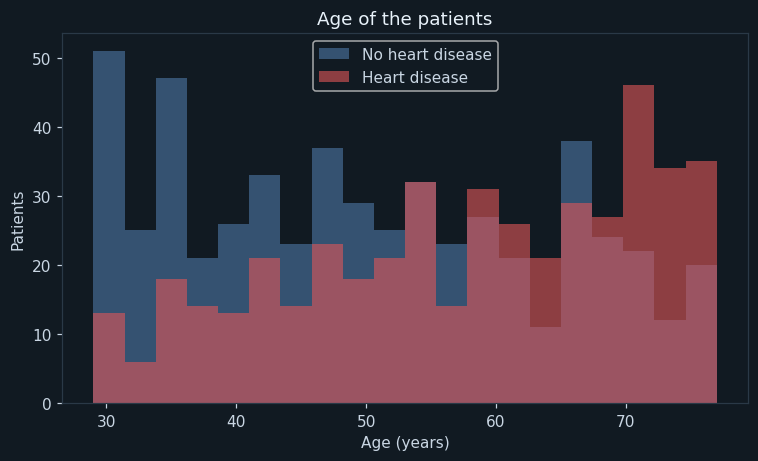
Two overlapping histograms: patients without (blue) and with (red) heart disease.
Patients with disease are older on average, but the two groups overlap heavily — age alone cannot separate them, and many younger patients have disease too.
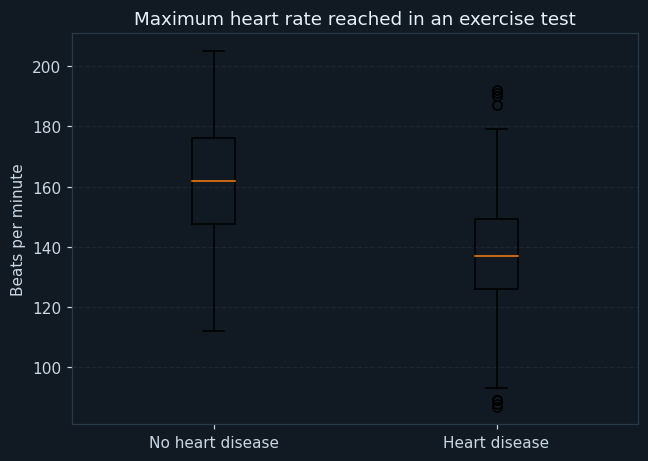
One box per group: the median heart rate reached, the middle half of patients, and the spread.
Patients with heart disease reach a lower maximum heart rate — a diseased heart cannot speed up as much under effort. The boxes overlap only partly, so this is one of the strongest single measurements.
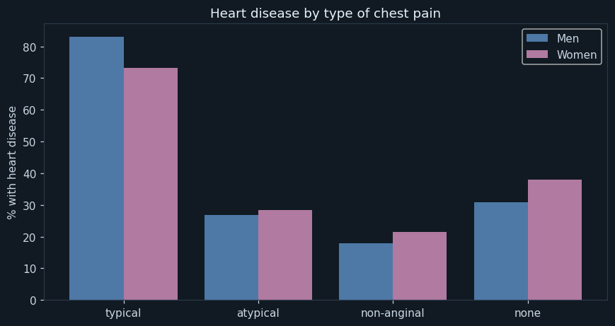
For each type of chest pain, the percentage of patients with heart disease — men and women separately.
Typical chest pain is a strong sign in both sexes, but it is a weaker one in women — and women with disease more often report atypical pain or none. A model leaning on typical pain will find men's disease more easily. This chart is the first warning of the fairness problem the Feedback step confirms.
7Step 6 — Data Preparation
drop_duplicates() removes them, so no patient appears in both training and testing data.
Replaced with a missing value and then filled with the median cholesterol. A new feature, cholesterol_missing, records which patients were untested — in case not being tested is itself informative.
Filled with the median blood pressure. Six rows is too few to drop good records for, and the median is not pulled by extreme readings.
sex becomes male = 1/0, exercise angina 1/0, and chest pain is one-hot encoded into four columns.
Feature engineering
Thirteen features go into the models. Besides encoding, one feature is created: cholesterol_missing. Feature engineering is not only transforming columns but asking what extra information is hidden in the data — here, the fact that a test was skipped.
Logistic Regression needs features on similar scales — heart rate in the hundreds should not outweigh ST depression in single figures. A StandardScaler is placed inside a scikit-learn Pipeline with the model, so the scaler learns its averages from the training data only. Scaling the whole dataset first would leak information from the test data into training.
Chart 4, a correlation heat map, checks that no two features are near-duplicates and shows which measurements move with disease.
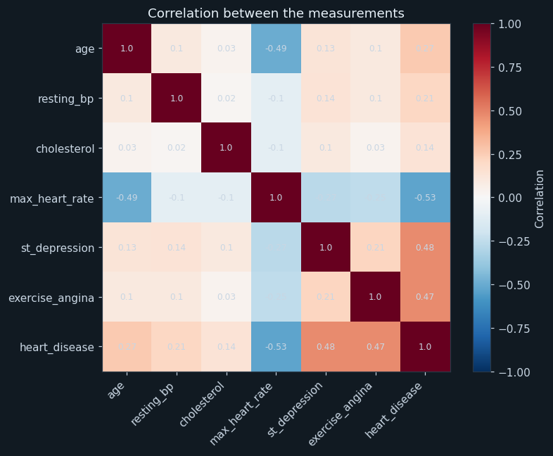
Each square is the correlation between two measurements, from −1 (blue) to +1 (red); the bottom row is correlation with heart disease.
ST depression and exercise angina correlate most strongly with disease, and maximum heart rate most strongly against it. Cholesterol correlates only weakly. No two features are near-duplicates, so all can stay.
8Step 7 — Modelling
Every training patient has a confirmed diagnosis, so this is supervised learning; the label has two classes, so it is binary classification.
The split uses stratify=y so that the training and testing sets have the same share of patients with disease as the whole dataset: 800 Testing rows : 200 patients for training and 200 for testing.
How the models work
Logistic Regression combines the features in a weighted sum, as linear regression does, but passes the result through an S-shaped curve that turns it into a probability between 0 and 1. The chart of its coefficients (chart 5) shows what it learned.
The Decision Tree splits the patients by yes/no questions — for example "is ST depression above 1.3?" — choosing at each step the question that best separates the two classes. max_depth=4 and min_samples_leaf=10 keep it small enough to explain and stop it memorising individual patients.
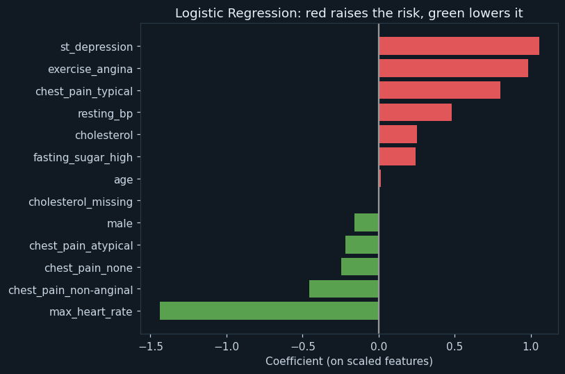
One coefficient per feature, on scaled features. Red bars raise the predicted risk, green bars lower it; longer bars matter more.
ST depression, exercise angina and typical chest pain raise the risk most; a high maximum heart rate lowers it most. These match medical knowledge, which is the first check that a model has learned something real rather than noise.
9Step 8 — Evaluation
On the 200 test patients, Logistic Regression's counts were 80 11 17 92 (TP, FN, FP, TN): accuracy 0.86, precision 0.825, recall 0.879, F1 0.851. The Decision Tree's were 76 15 16 93: accuracy 0.845, recall 0.835.
Stratified 5-fold cross validation, which keeps the share of disease the same in every fold, confirms the ranking: mean recall 0.855 for Logistic Regression against 0.784 for the Decision Tree.
Recall is the metric that matters most, as the doctor said in the interviews: a false negative is a patient with heart disease sent home. So the default threshold of 0.5 is lowered to 0.35. Recall rises to 0.923, precision stays at 0.808, and 104 of 200 test patients would be referred — a workload the cardiologist said was manageable.
Logistic Regression is chosen: higher recall, steadier across folds, and coefficients a doctor can understand.
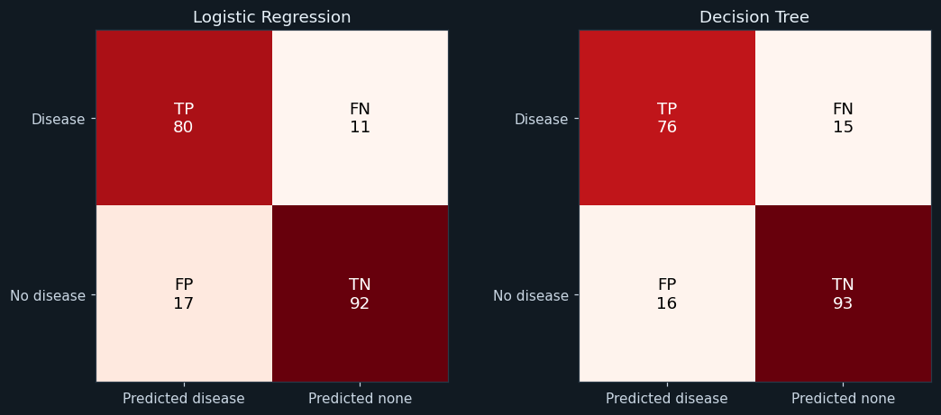
For each model, on the 200 test patients: TP (disease, flagged), FN (disease, missed), FP (healthy, flagged) and TN (healthy, cleared).
Logistic Regression has fewer false negatives — missed patients — than the Decision Tree, with about the same number of false positives. In screening, the FN box is the one to watch.
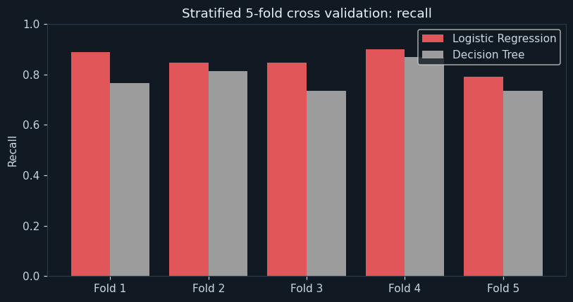
Recall of each model in each of the five stratified folds.
Logistic Regression's recall is higher than the tree's in every fold. The Decision Tree varies more from fold to fold — a sign it is more sensitive to which patients it happens to train on.
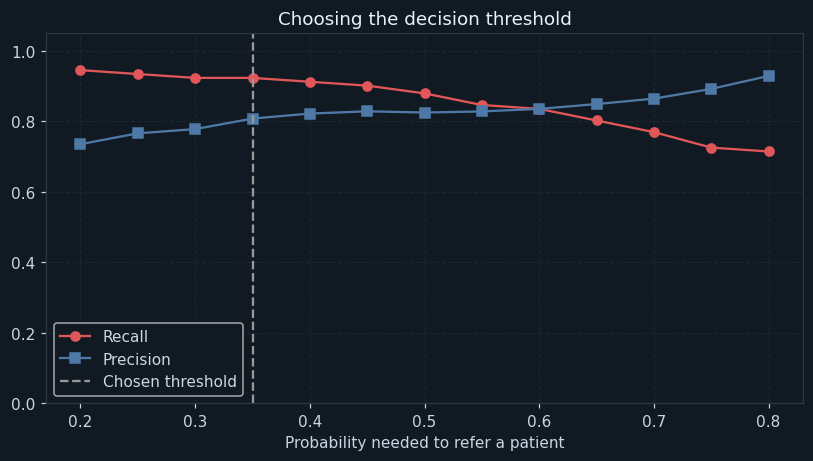
Recall (red) and precision (blue) of Logistic Regression if a patient is referred when their probability passes each threshold. The dashed line is the threshold chosen.
Lowering the threshold catches more patients with disease but refers more healthy ones. At 0.35, recall rises to 0.923 while precision stays at 0.808 — about half the patients are referred, roughly what the cardiologist said could be handled.
10Step 9 — Deployment
The pipeline — scaler and model together — is saved to heart_model.pkl, so new patients are scaled exactly as the training patients were. The program loads it and gives three new patients a probability and an action: refer at 0.35 or above, otherwise routine follow-up.
In a clinic, the doctor would enter the check-up results into a simple form and see the probability with the main reasons (from the coefficients). The doctor decides; the model only makes sure nobody at risk is overlooked in a busy queue.
11Step 10 — Feedback
Months later, the diagnoses of 200 more patients are confirmed. On them, the model's recall was 0.874 — close to the test result, so it still works overall.
But checked for men and women separately, recall was 0.889 for men and 0.833 for women — a gap of 5.6 points. The program's rule flags any gap above 5 points. The cause is the one chart 3 showed: in women, heart disease more often lacks typical chest pain and shows smaller ECG changes, so the features the model relies on are weaker signals for them.
The follow-up group is small — only 24 women with heart disease — so this is a warning to investigate, not proof. The right response is the methodology's loop back: collect more records from women, consider features that are better signals for them, and check again before the model is used widely.
12Ethical considerations
A missed patient can die. That is why recall, not accuracy, chose the threshold — the bioethics principle of non-maleficence applied to a metric.
A model that misses more women gives women worse care. The Feedback step checks recall by sex for exactly this reason, and found a gap. A fair model must be tested for each group it serves.
Patients decide about their own care. The model gives the doctor a probability and its reasons, so the doctor can explain it; it never gives a patient a verdict on its own.
Health records are among the most sensitive data there is. Real projects use anonymised public datasets; a school group must never collect real patient records.
13Source code
The whole program, laid out as the ten steps of the methodology. Every chart and number on this page came out of running it.
# ---------------------------------------------------------------------------
# heart_risk.py
#
# Capstone project: screening patients for heart disease from routine
# check-up measurements, so that those at risk are referred to a
# cardiologist early.
#
# CBSE Class XII, Artificial Intelligence (843), Part C - Capstone Project.
# SDG 3 (Good Health and Well-being).
#
# Data Science Methodology, 10 steps. A CLASSIFICATION problem: two models
# - Logistic Regression and a Decision Tree - compared with a train-test
# split and stratified 5-fold cross validation, using the confusion matrix,
# accuracy, precision, recall and F1. The decision threshold is then tuned,
# because in screening a missed patient costs far more than an extra test.
#
# Libraries: pandas, numpy, matplotlib, scikit-learn, joblib.
# ---------------------------------------------------------------------------

# %% Step 1 - Business Understanding
print("=" * 64)
print("WHO IS AT RISK OF HEART DISEASE?")
print("=" * 64)
print("Problem : heart disease is often found late; cardiologists are few")
print("Goal    : flag the patients at a check-up who should see a specialist")
print()

# %% Step 2 - Analytic Approach
print("Analytic approach : predictive - classification (disease: yes or no)")
print()

# %% Step 3 - Data Requirements
import pandas as pd
import numpy as np
import matplotlib.pyplot as plt
from sklearn.model_selection import train_test_split, StratifiedKFold, cross_validate
from sklearn.pipeline import make_pipeline
from sklearn.preprocessing import StandardScaler
from sklearn.linear_model import LogisticRegression
from sklearn.tree import DecisionTreeClassifier
from sklearn.metrics import confusion_matrix, accuracy_score, precision_score, recall_score, f1_score
import joblib

pd.set_option("display.width", 140)
pd.set_option("display.max_columns", 20)

# %% Step 4 - Data Collection
data = pd.read_csv("patients.csv")
print("Rows collected :", len(data))
print(data.head(6))
print()

# %% Step 5 - Data Understanding
print("--- Step 5: Data Understanding ---")
print("Missing values:")
print(data.isnull().sum().to_string())
print("Cholesterol recorded as 0 :", (data["cholesterol"] == 0).sum())
print()
print("Patients with and without heart disease:")
print(data["heart_disease"].value_counts().to_string())
print("Share with heart disease  :", round(data["heart_disease"].mean() * 100, 1), "%")
print()

sick = data[data["heart_disease"] == 1]
well = data[data["heart_disease"] == 0]

# Chart 1: age, with and without disease.
plt.figure(figsize=(7, 4.3))
plt.hist(well["age"], bins=20, alpha=0.6, color="#4e79a7", label="No heart disease")
plt.hist(sick["age"], bins=20, alpha=0.6, color="#e15759", label="Heart disease")
plt.title("Age of the patients")
plt.xlabel("Age (years)")
plt.ylabel("Patients")
plt.legend()
plt.tight_layout()
plt.savefig("chart1_age.png")
plt.close()

# Chart 2: maximum heart rate, as box plots.
plt.figure(figsize=(6, 4.3))
plt.boxplot([well["max_heart_rate"], sick["max_heart_rate"]], labels=["No heart disease", "Heart disease"])
plt.title("Maximum heart rate reached in an exercise test")
plt.ylabel("Beats per minute")
plt.grid(True, axis="y", linestyle="--", alpha=0.4)
plt.tight_layout()
plt.savefig("chart2_max_heart_rate.png")
plt.close()

# Chart 3: share with disease for each kind of chest pain, by sex.
share = data.groupby(["chest_pain", "sex"])["heart_disease"].mean().unstack() * 100
share = share.reindex(["typical", "atypical", "non-anginal", "none"])
print("Share with heart disease, by chest pain and sex (%):")
print(share.round(1))
print()
x = np.arange(4)
plt.figure(figsize=(8, 4.3))
plt.bar(x - 0.2, share["M"], width=0.4, label="Men", color="#4e79a7")
plt.bar(x + 0.2, share["F"], width=0.4, label="Women", color="#b07aa1")
plt.xticks(x, share.index)
plt.ylabel("% with heart disease")
plt.title("Heart disease by type of chest pain")
plt.legend()
plt.tight_layout()
plt.savefig("chart3_chest_pain.png")
plt.close()

# %% Step 6 - Data Preparation
print("--- Step 6: Data Preparation ---")
before = len(data)
data = data.drop_duplicates()
print("Duplicate rows removed               :", before - len(data))

# Cholesterol of 0 means "not measured", as in the UCI data it is modelled
# on. It is turned into a real missing value and then filled with the
# median - and a new column records that it was missing, in case being
# untested is itself informative.
data["cholesterol_missing"] = (data["cholesterol"] == 0).astype(int)
data["cholesterol"] = data["cholesterol"].replace(0, np.nan)
data["cholesterol"] = data["cholesterol"].fillna(data["cholesterol"].median())
data["resting_bp"] = pd.to_numeric(data["resting_bp"])
blank_bp = data["resting_bp"].isnull().sum()
data["resting_bp"] = data["resting_bp"].fillna(data["resting_bp"].median())
print("Cholesterol 0s replaced by the median:", data["cholesterol_missing"].sum())
print("Blank blood pressures filled         :", blank_bp)

data["male"] = (data["sex"] == "M").astype(int)
data["exercise_angina"] = (data["exercise_angina"] == "Yes").astype(int)
data = pd.get_dummies(data, columns=["chest_pain"], dtype=int)
features = ["age", "male", "resting_bp", "cholesterol", "cholesterol_missing", "fasting_sugar_high",
            "max_heart_rate", "exercise_angina", "st_depression", "chest_pain_atypical",
            "chest_pain_non-anginal", "chest_pain_none", "chest_pain_typical"]
print("Features used                        :", len(features))
print()

# Chart 4: correlations between the number features, as a heat map.
cols = ["age", "resting_bp", "cholesterol", "max_heart_rate", "st_depression", "exercise_angina", "heart_disease"]
corr = data[cols].corr()
plt.figure(figsize=(7.5, 6))
plt.imshow(corr, cmap="RdBu_r", vmin=-1, vmax=1)
plt.colorbar(label="Correlation")
plt.xticks(range(len(cols)), cols, rotation=45, ha="right")
plt.yticks(range(len(cols)), cols)
for i in range(len(cols)):
    for j in range(len(cols)):
        plt.text(j, i, round(corr.iloc[i, j], 2), ha="center", va="center", fontsize=8)
plt.title("Correlation between the measurements")
plt.tight_layout()
plt.savefig("chart4_heatmap.png")
plt.close()
print("Correlation with heart disease:")
print(corr["heart_disease"].drop("heart_disease").round(2).sort_values().to_string())
print()

# %% Step 7 - Modelling
print("--- Step 7: Modelling ---")
X = data[features]
y = data["heart_disease"]
# stratify=y keeps the same share of disease in the training and test sets.
X_train, X_test, y_train, y_test = train_test_split(X, y, test_size=0.2, stratify=y, random_state=11)
print("Training rows :", len(X_train), " Testing rows :", len(X_test))

# Logistic Regression needs features on similar scales, so a scaler is
# placed in front of it in a pipeline: the scaler learns only from the
# training data, and the test data is scaled with what it learned.
logistic = make_pipeline(StandardScaler(), LogisticRegression(max_iter=1000))
tree = DecisionTreeClassifier(max_depth=4, min_samples_leaf=10, random_state=0)
logistic.fit(X_train, y_train)
tree.fit(X_train, y_train)

coef = pd.Series(logistic[-1].coef_[0], index=features).sort_values()
print("Logistic Regression coefficients (scaled features):")
print(coef.round(2).to_string())
print()

# Chart 5: what Logistic Regression learned.
plt.figure(figsize=(7.5, 5))
plt.barh(coef.index, coef.values, color=["#59a14f" if v < 0 else "#e15759" for v in coef.values])
plt.axvline(0, color="#999999")
plt.title("Logistic Regression: red raises the risk, green lowers it")
plt.xlabel("Coefficient (on scaled features)")
plt.tight_layout()
plt.savefig("chart5_coefficients.png")
plt.close()

# %% Step 8 - Evaluation
print("--- Step 8: Evaluation ---")
for name, model in [["Logistic Regression", logistic], ["Decision Tree", tree]]:
    pred = model.predict(X_test)
    tn, fp, fn, tp = confusion_matrix(y_test, pred).ravel()
    print(name)
    print("  " + name + " TP, FN, FP, TN :", tp, fn, fp, tn)
    print("  " + name + " accuracy  :", round(accuracy_score(y_test, pred), 3))
    print("  " + name + " precision :", round(precision_score(y_test, pred), 3))
    print("  " + name + " recall    :", round(recall_score(y_test, pred), 3))
    print("  " + name + " F1        :", round(f1_score(y_test, pred), 3))
print()

# Stratified 5-fold cross validation: every fold keeps the same share of
# patients with disease as the whole dataset.
folds = StratifiedKFold(n_splits=5, shuffle=True, random_state=1)
cv = {}
for name, model in [["Logistic Regression", make_pipeline(StandardScaler(), LogisticRegression(max_iter=1000))],
                    ["Decision Tree", DecisionTreeClassifier(max_depth=4, min_samples_leaf=10, random_state=0)]]:
    scores = cross_validate(model, X, y, cv=folds, scoring=["accuracy", "recall"])
    cv[name] = scores
    print(name, "- recall in each fold   :", np.round(scores["test_recall"], 3))
    print(name, "- mean CV accuracy      :", round(scores["test_accuracy"].mean(), 3))
    print(name, "- mean CV recall        :", round(scores["test_recall"].mean(), 3))
print()

# Chart 6: both confusion matrices.
plt.figure(figsize=(10, 4.3))
for k, (name, model) in enumerate([["Logistic Regression", logistic], ["Decision Tree", tree]]):
    m = confusion_matrix(y_test, model.predict(X_test), labels=[1, 0])
    plt.subplot(1, 2, k + 1)
    plt.imshow(m, cmap="Reds")
    labels = [["TP", "FN"], ["FP", "TN"]]
    for r in range(2):
        for c in range(2):
            plt.text(c, r, labels[r][c] + "\n" + str(m[r][c]), ha="center", va="center", fontsize=12,
                     color="white" if m[r][c] > m.max() / 2 else "black")
    plt.xticks([0, 1], ["Predicted disease", "Predicted none"])
    plt.yticks([0, 1], ["Disease", "No disease"])
    plt.title(name)
plt.tight_layout()
plt.savefig("chart6_confusion.png")
plt.close()

# Chart 7: recall in each fold.
x = np.arange(5)
plt.figure(figsize=(7.5, 4))
plt.bar(x - 0.2, cv["Logistic Regression"]["test_recall"], width=0.4, label="Logistic Regression", color="#e15759")
plt.bar(x + 0.2, cv["Decision Tree"]["test_recall"], width=0.4, label="Decision Tree", color="#9c9c9c")
plt.xticks(x, ["Fold 1", "Fold 2", "Fold 3", "Fold 4", "Fold 5"])
plt.ylim(0, 1)
plt.ylabel("Recall")
plt.title("Stratified 5-fold cross validation: recall")
plt.legend()
plt.tight_layout()
plt.savefig("chart7_kfold_recall.png")
plt.close()

# The threshold. Logistic Regression gives each patient a probability;
# by default a patient is flagged at 0.5. A lower threshold catches more
# patients with disease (recall up) at the cost of more referrals that
# turn out healthy (precision down).
prob = logistic.predict_proba(X_test)[:, 1]
thresholds = np.round(np.arange(0.2, 0.81, 0.05), 2)
prec_list = []
rec_list = []
for t in thresholds:
    flag = (prob >= t).astype(int)
    prec_list.append(precision_score(y_test, flag, zero_division=0))
    rec_list.append(recall_score(y_test, flag))
chosen = 0.35
flag = (prob >= chosen).astype(int)
print("Threshold chosen for screening   :", chosen)
print("Recall at threshold 0.35         :", round(recall_score(y_test, flag), 3))
print("Precision at threshold 0.35      :", round(precision_score(y_test, flag), 3))
print("Patients referred at 0.35        :", flag.sum(), "of", len(flag))
print()

# Chart 8: precision and recall at every threshold.
plt.figure(figsize=(7.5, 4.3))
plt.plot(thresholds, rec_list, marker="o", color="#e15759", label="Recall")
plt.plot(thresholds, prec_list, marker="s", color="#4e79a7", label="Precision")
plt.axvline(chosen, color="#999999", linestyle="--", label="Chosen threshold")
plt.title("Choosing the decision threshold")
plt.xlabel("Probability needed to refer a patient")
plt.ylim(0, 1.05)
plt.legend()
plt.grid(True, linestyle="--", alpha=0.4)
plt.tight_layout()
plt.savefig("chart8_threshold.png")
plt.close()

# %% Step 9 - Deployment
print("--- Step 9: Deployment ---")
joblib.dump(logistic, "heart_model.pkl")
model = joblib.load("heart_model.pkl")
new_patients = pd.DataFrame({
    "age": [62, 45, 51], "male": [1, 0, 1], "resting_bp": [150, 120, 135], "cholesterol": [290, 210, 245],
    "cholesterol_missing": [0, 0, 0], "fasting_sugar_high": [1, 0, 0], "max_heart_rate": [118, 172, 150],
    "exercise_angina": [1, 0, 0], "st_depression": [2.4, 0.2, 1.0], "chest_pain_atypical": [0, 1, 0],
    "chest_pain_non-anginal": [0, 0, 1], "chest_pain_none": [0, 0, 0], "chest_pain_typical": [1, 0, 0],
})
p_new = model.predict_proba(new_patients)[:, 1]
for i in range(len(new_patients)):
    if p_new[i] >= chosen:
        action = "REFER to a cardiologist"
    else:
        action = "routine follow-up"
    print("Patient", i + 1, "- probability", round(p_new[i], 3), "->", action)
print()

# %% Step 10 - Feedback
print("--- Step 10: Feedback ---")
# Months later, the diagnoses of 200 more patients are confirmed. Checking
# the model against them - for men and women separately - shows whether it
# works equally well for everyone.
fu = pd.read_csv("follow_up.csv")
fu["cholesterol_missing"] = 0
fu["male"] = (fu["sex"] == "M").astype(int)
fu["exercise_angina"] = (fu["exercise_angina"] == "Yes").astype(int)
fu = pd.get_dummies(fu, columns=["chest_pain"], dtype=int)
fu_flag = (model.predict_proba(fu[features])[:, 1] >= chosen).astype(int)
print("Follow-up patients                :", len(fu))
print("Recall on follow-up, everyone     :", round(recall_score(fu["heart_disease"], fu_flag), 3))
men = fu["male"] == 1
print("Recall on follow-up, men          :", round(recall_score(fu["heart_disease"][men], fu_flag[men]), 3))
print("Recall on follow-up, women        :", round(recall_score(fu["heart_disease"][~men], fu_flag[~men]), 3))
gap = recall_score(fu["heart_disease"][men], fu_flag[men]) - recall_score(fu["heart_disease"][~men], fu_flag[~men])
print("Recall gap, men minus women       :", round(gap * 100, 1), "points")
if gap > 0.05:
    print("Feedback: the model misses more women than men - collect more records")
    print("          from women and review the features before wider use.")
else:
    print("Feedback: recall is similar for men and women.")
The library calls it is built from
| Call | Step | What it does |
|---|---|---|
pd.read_csv() / isnull().sum() | Steps 4–5 | Reads the records and counts missing values |
groupby([...]).mean().unstack() | Step 5 | Share with disease by chest pain and sex |
replace(0, np.nan) / fillna(median) | Step 6 | Turns cholesterol 0 into missing, then fills it |
pd.get_dummies() | Step 6 | One-hot encodes chest pain |
train_test_split(stratify=y) | Step 7 | Keeps the share of disease equal in both sets |
make_pipeline(StandardScaler(), LogisticRegression()) | Step 7 | Scales inside the model, without leaking test data |
DecisionTreeClassifier(max_depth=4) | Step 7 | A small, explainable tree |
confusion_matrix / precision_score / recall_score / f1_score | Step 8 | The classification metrics |
StratifiedKFold + cross_validate() | Step 8 | Stratified 5-fold cross validation |
predict_proba() | Steps 8–10 | Each patient's probability, for the threshold |
joblib.dump() / load() | Step 9 | Saves and reloads the whole pipeline |
14Output of a real run
================================================================
WHO IS AT RISK OF HEART DISEASE?
================================================================
Problem : heart disease is often found late; cardiologists are few
Goal    : flag the patients at a check-up who should see a specialist

Analytic approach : predictive - classification (disease: yes or no)

Rows collected : 1003
  patient_id  age sex   chest_pain  resting_bp  cholesterol  fasting_sugar_high  max_heart_rate exercise_angina  st_depression  \
0     H40001   49   F         none       126.0        230.0                   0           164.0              No            0.8
1     H40002   39   F  non-anginal       144.0        250.0                   0           145.0              No            1.3
2     H40003   71   M  non-anginal       117.0        217.0                   0           174.0              No            0.0
3     H40004   49   M      typical       147.0        273.0                   1           131.0             Yes            2.1
4     H40005   52   M      typical       163.0        278.0                   0           124.0             Yes            1.7
5     H40006   68   M     atypical       127.0        260.0                   0           152.0              No            1.2

   heart_disease
0              0
1              0
2              0
3              1
4              1
5              0

--- Step 5: Data Understanding ---
Missing values:
patient_id            0
age                   0
sex                   0
chest_pain            0
resting_bp            6
cholesterol           0
fasting_sugar_high    0
max_heart_rate        0
exercise_angina       0
st_depression         0
heart_disease         0
Cholesterol recorded as 0 : 37

Patients with and without heart disease:
heart_disease
0    547
1    456
Share with heart disease  : 45.5 %

Share with heart disease, by chest pain and sex (%):
sex             F     M
chest_pain
typical      73.2  83.1
atypical     28.3  26.8
non-anginal  21.5  17.9
none         38.0  30.8

--- Step 6: Data Preparation ---
Duplicate rows removed               : 3
Cholesterol 0s replaced by the median: 37
Blank blood pressures filled         : 6
Features used                        : 13

Correlation with heart disease:
max_heart_rate    -0.53
cholesterol        0.14
resting_bp         0.21
age                0.27
exercise_angina    0.47
st_depression      0.48

--- Step 7: Modelling ---
Training rows : 800  Testing rows : 200
Logistic Regression coefficients (scaled features):
max_heart_rate           -1.44
chest_pain_non-anginal   -0.45
chest_pain_none          -0.25
chest_pain_atypical      -0.22
male                     -0.16
cholesterol_missing       0.00
age                       0.02
fasting_sugar_high        0.24
cholesterol               0.25
resting_bp                0.48
chest_pain_typical        0.80
exercise_angina           0.98
st_depression             1.05

--- Step 8: Evaluation ---
Logistic Regression
  Logistic Regression TP, FN, FP, TN : 80 11 17 92
  Logistic Regression accuracy  : 0.86
  Logistic Regression precision : 0.825
  Logistic Regression recall    : 0.879
  Logistic Regression F1        : 0.851
Decision Tree
  Decision Tree TP, FN, FP, TN : 76 15 16 93
  Decision Tree accuracy  : 0.845
  Decision Tree precision : 0.826
  Decision Tree recall    : 0.835
  Decision Tree F1        : 0.831

Logistic Regression - recall in each fold   : [0.889 0.846 0.846 0.901 0.791]
Logistic Regression - mean CV accuracy      : 0.866
Logistic Regression - mean CV recall        : 0.855
Decision Tree - recall in each fold   : [0.767 0.813 0.736 0.868 0.736]
Decision Tree - mean CV accuracy      : 0.829
Decision Tree - mean CV recall        : 0.784

Threshold chosen for screening   : 0.35
Recall at threshold 0.35         : 0.923
Precision at threshold 0.35      : 0.808
Patients referred at 0.35        : 104 of 200

--- Step 9: Deployment ---
Patient 1 - probability 0.999 -> REFER to a cardiologist
Patient 2 - probability 0.012 -> routine follow-up
Patient 3 - probability 0.084 -> routine follow-up

--- Step 10: Feedback ---
Follow-up patients                : 200
Recall on follow-up, everyone     : 0.874
Recall on follow-up, men          : 0.889
Recall on follow-up, women        : 0.833
Recall gap, men minus women       : 5.6 points
Feedback: the model misses more women than men - collect more records
from women and review the features before wider use.15The same project in Orange
Unit 4 of the curriculum teaches classification and its evaluation in Orange; this project maps onto those widgets directly. The tool is Orange Data Mining.
| Widget | What it does |
|---|---|
| File | Load patients.csv; set heart_disease as the target and patient_id as meta. |
| Edit Domain + Impute | Treat cholesterol 0 as missing; impute with the median. |
| Distributions / Box Plot | Compare age and maximum heart rate for the two classes. |
| Logistic Regression and Tree | The two learners; set the tree's depth to 4. |
| Test and Score | Stratified 5-fold cross validation; read CA, precision, recall and F1 with target class 1. |
| Confusion Matrix | Count the false negatives for each model. |
| ROC Analysis | See the trade-off between catching patients and false alarms across all thresholds. |
16Testing
Every case was run: each gives the whole program a small input of its own.
| Test case | Expected | Actual | Result |
|---|---|---|---|
| The full dataset | Rows collected : 1003 | Rows collected : 1003 | Pass |
| Three duplicated patients are removed | Duplicate rows removed : 3 | Duplicate rows removed : 3 | Pass |
| Cholesterol of 0 means not measured: 37 replaced | Cholesterol 0s replaced by the median: 37 | Cholesterol 0s replaced by the median: 37 | Pass |
| Lowering the threshold to 0.35 raises recall | Recall at threshold 0.35 : 0.923 | Recall at threshold 0.35 : 0.923 | Pass |
| Feedback finds the model misses more women | Recall gap, men minus women : 5.6 points | Recall gap, men minus women : 5.6 points | Pass |
| Sick and healthy patients that never overlap: no patient missed | Logistic Regression recall : 1.0 | Logistic Regression recall : 1.0 | Pass |
| Five cholesterol values of 0 are all treated as missing | Cholesterol 0s replaced by the median: 5 | Cholesterol 0s replaced by the median: 5 | Pass |
| The data file is missing | FileNotFoundError: [Errno 2] No such file or directory: 'patients.csv' | FileNotFoundError: [Errno 2] No such file or directory: 'patients.csv' | Pass |
17Team roles and timeline
A capstone is done by a group of 3 to 5. A suggested split of the work, and a timeline across the year:
| Role | Responsible for |
|---|---|
| Project lead | Business understanding; interviews with the doctor and cardiologist; presentation |
| Data lead | Choosing and documenting the public dataset; data requirements; privacy |
| Analyst | Data understanding and preparation, including the cholesterol-0 problem |
| Modeller | The two models, cross validation, and the threshold |
| Ethics and documentation | The fairness check, the ethics section, the report and the video |
| When | Methodology steps | Deliverable |
|---|---|---|
| April – May | 1 Business Understanding, 2 Analytic Approach | Problem statement; interviews |
| June – July | 3 Data Requirements, 4 Data Collection | Public dataset chosen and documented |
| August | 5 Data Understanding, 6 Data Preparation | Clean data; exploratory charts |
| September – October | 7 Modelling, 8 Evaluation | Models compared; threshold chosen |
| November | 9 Deployment, 10 Feedback | Saved model; fairness check on follow-up data |
| December – January | Documentation and video | Report and 3-minute video |
18Results, limits and what next
- Logistic Regression screens with recall 0.879 at the default threshold, better than the Decision Tree's 0.835.
- Stratified 5-fold cross validation confirms it: mean recall 0.855 against 0.784.
- Lowering the threshold to 0.35 raises recall to 0.923 with precision 0.808.
- ST depression, exercise angina, typical chest pain and a low maximum heart rate are the strongest signals — matching medical knowledge.
- On follow-up patients the model missed more women than men — a 5.6 points gap — because women's disease more often lacks the typical signs.
Limitations
- Sample data modelled on a public dataset; real clinical use would need validation on real patients
- Few women with disease in the follow-up, so the fairness gap is uncertain
- No smoking, family history or diabetes duration — all known risk factors
- Requires an exercise test, which not every check-up includes
Future scope
- Collect more data from women and older diabetic patients, and recheck recall for each group
- Add smoking and family history as features
- Build a version for check-ups without an exercise test
- Report an ROC curve and choose the threshold with the clinicians
What the team had to learn
- Logistic Regression and probabilities; decision trees
- Precision, recall and the decision threshold
- Stratified splitting and stratified K-fold cross validation
- Pipelines, and why scaling must be fitted on training data only
- Checking a model's fairness group by group
19Conclusion
The capstone built a heart-disease screening model that, with a threshold tuned for recall, catches about nine in ten patients with disease while referring a number of patients a cardiologist can see. Logistic Regression beat the Decision Tree on recall and was steadier across folds.
The Feedback step found the most important result: the model misses more women than men, because their disease less often shows the typical signs it relies on. Overall accuracy hid this completely. Only checking each group separately revealed it.
A screening model in healthcare is never finished at deployment. Following the methodology's feedback loop — and the bioethics principle of justice — means collecting better data for the group it serves worst, and checking again.
20The 3-minute video script
Part C asks for a video of exactly three minutes with six parts. A script, timed to the second:
| Time | Part | What to say and show |
|---|---|---|
| 0:00 – 0:25 | a. Problem statement | "Heart disease is India's biggest killer, and it is often found only after a heart attack. Doctors at check-ups have minutes to decide who sees a cardiologist." |
| 0:25 – 0:40 | b. SDG alignment | SDG 3 icon. "Target 3.4: cut early deaths from diseases like heart disease by a third." |
| 0:40 – 1:15 | c. AI concepts and algorithms | "Predictive analytics with binary classification. We compared Logistic Regression and a Decision Tree, using stratified 5-fold cross validation, and judged them by recall — because a missed patient is the worst mistake." |
| 1:15 – 2:15 | d. How it works | Show the cholesterol-0 cleaning, the confusion matrices, the threshold chart, and three new patients being scored. Then the follow-up check: recall for men and women. |
| 2:15 – 2:45 | e. Conclusion | "Our model catches about nine in ten patients with disease — but it misses more women. The next step is better data for women." |
| 2:45 – 3:00 | f. Acknowledgement | "We thank our AI teacher, [name], and the doctors who advised us." |
21Questions for the viva
▸Why is recall more important than accuracy in your project?
A false negative is a patient with heart disease who is not referred and may have a heart attack. Recall measures how many patients with disease are caught.
▸What did you do with cholesterol values of 0?
A cholesterol of 0 is impossible, so it means not measured. We made it missing, filled it with the median, and added a feature recording that it was missing.
▸Why did you use stratify=y and StratifiedKFold?
To keep the same share of patients with disease in the training data, the test data and every fold, so no split is unrepresentative by chance.
▸Why is the scaler inside a pipeline?
So it learns its averages from the training data only. Scaling the whole dataset first would leak information from the test data into training.
▸Why did you lower the threshold to 0.35?
To catch more patients with disease. Recall rose while precision fell only a little, and the number of referrals stayed manageable.
▸What did the Feedback step find?
Recall was lower for women than men, because women's heart disease more often lacks typical chest pain and large ECG changes.
▸Which bioethics principles apply?
Non-maleficence — avoid harm, so high recall — and justice — the model must work fairly for every group.
▸Which SDG does it align to?
SDG 3, Good Health and Well-being, target 3.4.
22References
- Janosi, A., Steinbrunn, W., Pfisterer, M. and Detrano, R. (1988). Heart Disease dataset (Cleveland), UCI Machine Learning Repository — https://archive.ics.uci.edu/dataset/45/heart+disease
- World Health Organization — Cardiovascular diseases fact sheet and HEARTS technical package — https://www.who.int/
- Mehta, L. S. et al. (2016). Acute Myocardial Infarction in Women: A Scientific Statement From the American Heart Association. Circulation, 133(9).
- scikit-learn user guide: Logistic Regression, Decision Trees, Pipelines, StratifiedKFold — https://scikit-learn.org/stable/user_guide.html
- CBSE, Artificial Intelligence (Subject Code 843), Class XII curriculum, 2026-27 — Part C
- CBSE, Artificial Intelligence Student Handbook, Class XII — Unit 2, Data Science Methodology
- Rollins, J. B. (2015). Foundational Methodology for Data Science. IBM Analytics.
- scikit-learn — https://scikit-learn.org/stable/; pandas, NumPy and Matplotlib documentation
- LambdaLab — https://www.lambdalab.in