Tomorrow's Electricity Demand
Forecasting a city's daily peak demand from weather and the calendar — Linear Regression, a Random Forest and a neural network, tested on a year they never saw, cross-validated through time, and caught drifting by the feedback step.
1Introduction
Electricity cannot be stored in large amounts, so supply must match demand every moment. Each afternoon a distribution company decides how much power to schedule for the next day, from its own plants and from the power exchange.
Get it wrong one way and there is load-shedding in a heatwave. Get it wrong the other way and the company pays for expensive power it does not need. Either way, consumers pay — in blackouts or in bills.
Tomorrow's demand depends on things known today: the weather forecast, whether tomorrow is a Sunday or a holiday, and how much power was used yesterday and last week. This capstone builds a day-ahead forecast from them, following the Data Science Methodology — and, as forecasting demands, tests it only on days in the future.
Affordable and Clean Energy
Climate Action
SDG 7 asks for affordable, reliable power for everyone. A distribution company buys most of tomorrow's power today; if it under-buys, homes face load-shedding, and if it over-buys, it pays for power nobody uses — and passes the cost on. A good demand forecast keeps the lights on at the lowest cost, and lets the grid plan around solar and wind instead of keeping extra coal plants running just in case, which is SDG 13.
2Step 1 — Business Understanding
What is the problem that you are trying to solve? The handbook uses the 5W1H Problem Canvas for this step.
- • The distribution company's load-dispatch team
- • Households and businesses who face blackouts or higher bills
- • Tomorrow's demand must be guessed today
- • Errors mean load-shedding or wasted, expensive power
- • One city's electricity distribution network
- • Every afternoon, for the next day's peak
- • Most critically in summer heatwaves
- • Reliable supply at the lowest cost
- • Better planning lets more solar and wind into the grid
- • Learn how demand depends on weather, calendar and recent demand
- • Forecast each day from the information known the day before
Problem statement
Who would use it: The load-dispatch team of a city's electricity distribution company, who schedule and buy tomorrow's power each afternoon.
Talking to the stakeholders
The handbook pairs the 5W1H canvas with Design Thinking, which begins by empathising with the people who have the problem. The questions asked, and what each answer changed:
| Question asked | What we learned, and what it changed |
|---|---|
| To a load dispatcher: what do you look at to plan tomorrow? | Yesterday's demand, the same day last week, and the temperature forecast. Those became the core features — and the rule that every feature must be known the day before. |
| To the same dispatcher: when are your forecasts worst? | Heatwaves, holidays and the first hot days of the year. So the data needed a holiday flag and a feature for heat above the point where air-conditioners switch on. |
| To a dispatcher: how close does a forecast need to be? | Within about 5% of demand is good; 10% causes problems. That became the evaluation yardstick: RMSE as a percentage of average demand. |
| To an energy auditor: is the meter data reliable? | There are gaps when meters fail, and on a grid-failure day the meters read zero. Both had to be handled in data preparation — and a zero is not a real demand. |
| To a consumer: what do you notice when forecasts go wrong? | Power cuts in May and June. That made summer the period to examine most closely (chart 7). |
| To an engineer: does demand change from year to year? | It grows several per cent a year as the city grows. A warning that a model trained on old years may drift — which the Feedback step later confirmed. |
How it is handled today
The simplest forecast, and not a bad one, because demand changes slowly. It fails on Mondays after a quiet Sunday, on holidays and at the start of a heatwave. It is the baseline every model here must beat.
Experienced dispatchers adjust for weather and holidays well, but the judgement is hard to pass on and hard to check.
Regional load-dispatch centres forecast demand for whole states. A city distribution company still needs its own, more detailed forecast.
Objectives
- To frame day-ahead demand forecasting with the 5W1H canvas
- To collect and understand three years of daily demand with weather and calendar data
- To prepare the data: remove duplicate dates, treat a grid failure as missing, interpolate gaps, and engineer lag and heat features
- To train Linear Regression, a Random Forest and a neural network on 2022–2023 and test them on 2024
- To compare them with time-series cross validation, which never tests on the past
- To deploy the chosen model for a day-ahead forecast, and use January 2025 as feedback
3Step 2 — Analytic Approach
Forecasting tomorrow's demand from past patterns is predictive analytics; the target is a number of megawatts, so the technique is regression. Because the rows are days in order, it is regression on a time series, which changes how the data must be split: the model must always be tested on days later than those it learned from.
The forecast feeds a prescriptive decision — how much power to schedule — which the dispatchers make.
| Candidate | Why it was considered |
|---|---|
| Linear Regression | Explainable: each coefficient says how many megawatts a degree of heat or a Sunday adds or removes. |
| Random Forest Regressor | Can follow curved effects such as air-conditioning load rising faster in extreme heat; cannot predict beyond the range of values it was trained on. |
| Neural Network (MLP Regressor) | A multi-layer perceptron with two hidden layers (32 and 16 neurons), as introduced in Unit 6. Flexible, but needs more data and is harder to explain. |
| Same as yesterday (baseline) | Not a model to deploy — the benchmark that shows whether the models add anything. |
4Step 3 — Data Requirements
Every feature must be known by the afternoon before the day being forecast. Tomorrow's actual temperature is not known — so in real use the weather feature is the weather forecast. Yesterday's demand is known; tomorrow's is what we are predicting.
At least two full years are needed, so that every season appears in the training data, plus a later period to test on.
| Data needed | Type | Format | Source |
|---|---|---|---|
| Date | Date | YYYY-MM-DD, one row per day | Distribution company |
| Daily peak demand (target) | Numeric | Megawatts | SCADA / meter data, distribution company |
| Maximum temperature | Numeric | °C | India Meteorological Department |
| Humidity | Numeric | % | India Meteorological Department |
| Holiday | Binary | 1 / 0 | Government holiday list |
| Day of week, month | Derived | From the date | Engineered in Step 6 |
5Step 4 — Data Collection
Demand data is secondary data held by the distribution company (from its SCADA system and meters); weather data comes from the India Meteorological Department; holidays from the government calendar. For a real capstone, Grid-India publishes daily demand for each state and many state load-dispatch centres publish daily reports.
The sample file, power_demand.csv, holds 1097 rows from 2022-01-01 to 2024-12-31. january_2025.csv holds the following month and is used only in the Feedback step.
| Column | Type | What it holds | Role |
|---|---|---|---|
date | date | The day | used to make features and to split |
max_temp_c | decimal | Maximum temperature, °C | feature |
humidity_pct | integer | Relative humidity, % | feature |
holiday | 0 / 1 | 1 on a public holiday | feature |
demand_mw | decimal | Daily peak demand, MW | target |
cooling_degrees | decimal | Degrees above 27 °C — made by the program | engineered feature |
is_saturday, is_sunday, month | integer | From the date — made by the program | engineered features |
demand_yesterday, demand_last_week | decimal | Demand 1 and 7 days earlier — made by the program | engineered (lag) features |
power_demand.csv — Three years of daily peak demand, temperature, humidity and holidays for one city. 1,097 rows, 32.1 KB. Download the file
january_2025.csv — The following month, used only for feedback. 31 rows, 1.0 KB. Download the file
The first eight rows of power_demand.csv
| date | max_temp_c | humidity_pct | holiday | demand_mw |
|---|---|---|---|---|
2022-01-01 | 23.0 | 50.0 | 0 | 3782.0 |
2022-01-02 | 23.4 | 71.0 | 0 | 3616.0 |
2022-01-03 | 22.4 | 73.0 | 0 | 3749.0 |
2022-01-04 | 21.4 | 43.0 | 0 | 3738.0 |
2022-01-05 | 22.1 | 57.0 | 0 | 3735.0 |
2022-01-06 | 21.2 | 75.0 | 0 | 3892.0 |
2022-01-07 | 22.8 | 61.0 | 0 | 3768.0 |
2022-01-08 | 24.8 | 57.0 | 0 | 3607.0 |
The first four rows of january_2025.csv
| date | max_temp_c | humidity_pct | holiday | demand_mw |
|---|---|---|---|---|
2025-01-01 | 19.4 | 56.0 | 0 | 4296.0 |
2025-01-02 | 22.9 | 57.0 | 0 | 4422.0 |
2025-01-03 | 22.0 | 56.0 | 0 | 4221.0 |
2025-01-04 | 21.0 | 61.0 | 0 | 4156.0 |
6Step 5 — Data Understanding
Is the data collected representative of the problem to be solved?
Three checks: is every day present, are the readings believable, and do the features relate to demand? The data has a few blank days, one day recorded as 0 MW — impossible for a city, so a grid failure — and one date entered twice.
Chart 1 shows three things at once: a strong yearly cycle peaking in May–June, a slow rise from year to year, and the grid-failure day as a spike to zero. Chart 2 shows that demand barely changes with temperature until about 27–28 °C and then rises steeply — air-conditioners switching on. Chart 3 shows Sundays, and to a lesser extent Saturdays, well below weekdays.
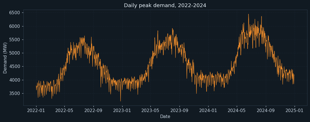
Peak demand for every day of the three years.
Demand rises to a peak every May–June and falls to a low in winter, and each year's line sits a little higher than the last — the city is growing. The single drop to zero is the grid-failure day, which Step 6 removes.
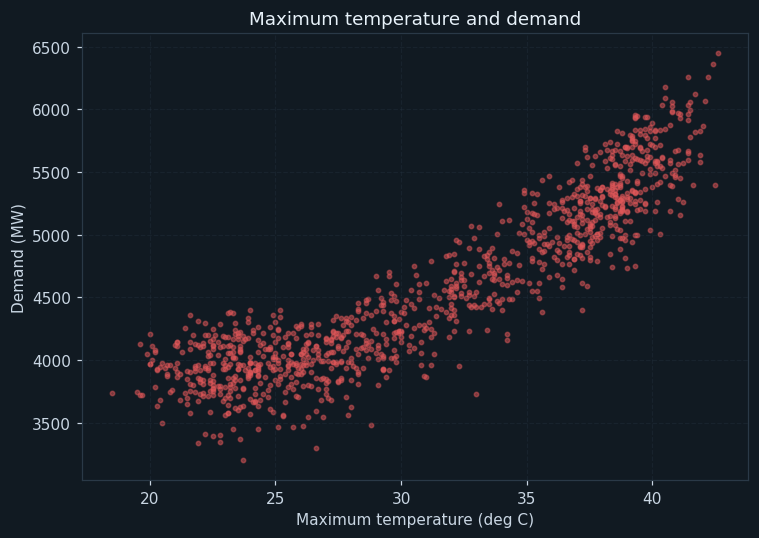
Each dot is a day: maximum temperature across, demand up.
Below about 27 °C, temperature hardly matters. Above it, demand climbs steeply, and faster still in extreme heat. That bend is why a cooling_degrees feature was engineered: a straight line through all the dots would get both cool and hot days wrong.
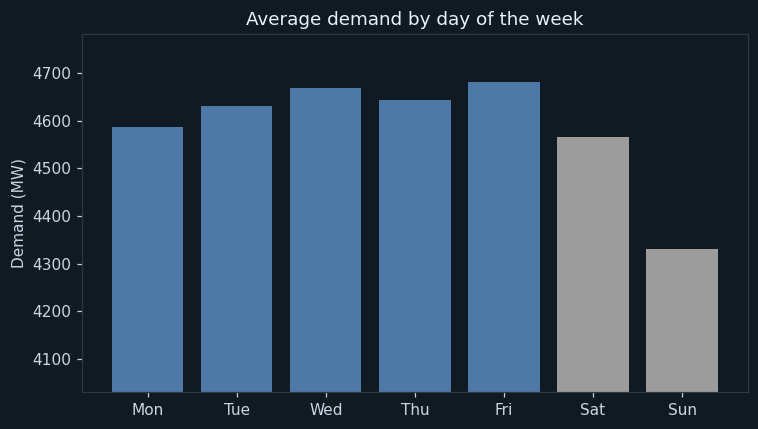
Average demand for each weekday over the three years. The axis does not start at zero, to make the differences visible — the bars compare days, not totals.
Sunday demand is far below the weekdays and Saturday's somewhat below, as offices and factories close. Monday's forecast is the hardest for 'same as yesterday', because yesterday was a Sunday.
7Step 6 — Data Preparation
Duplicates are removed by date, and the series is sorted by date, so each day appears once and in order.
Zero is not a real demand: the meters stopped. It is turned into a missing value, so it cannot drag the model down.
Filled by interpolation — a straight line between the days either side. For a smooth day-to-day series this is far better than filling with the overall average, which would ignore the season.
Feature engineering
Feature engineering carries this project. cooling_degrees is the heat above 27 °C (zero below it), because chart 2 shows air-conditioning load starts there; a straight-line model can use it to bend its temperature effect. is_saturday and is_sunday capture the weekly pattern, and month the season.
The two lag features, demand_yesterday and demand_last_week, are created with shift(). They carry the momentum of demand and its weekly rhythm — and they are known the day before, so using them is not cheating. The first seven days have no 'last week' and are dropped, leaving 1089 (first 7 days have no 'last week').
Chart 4 shows the monthly pattern the month feature captures.
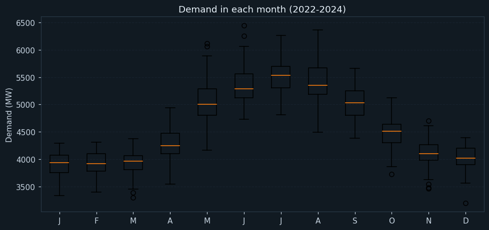
One box per month over the three years: median, middle half and spread.
May and June are the highest and most variable months — exactly where forecasting matters most and goes wrong most often. Winter months are low and steady.
8Step 7 — Modelling
Each training day has its actual demand — the label — so this is supervised regression. The split is by time, not random: 723 days of 2022–2023 for training and 366 days of 2024 for testing. Shuffling would let the model learn from days after those it is tested on, which is impossible in real forecasting.
Three models are trained on exactly the same features.
How the models work
Linear Regression learns one coefficient per feature. Its coefficients read like a dispatcher's rules of thumb: each degree of heat above 27 °C adds about 78 MW, a Sunday removes about 290 MW and a holiday about 457 MW, and yesterday's demand carries over with a weight of about 0.34.
The Random Forest averages 300 decision trees, each splitting the days by questions such as "is cooling_degrees above 6?"
The neural network is a multi-layer perceptron, the network type introduced in Unit 6: 9 inputs, a hidden layer of 32 neurons, a second of 16, and one output. Each neuron computes a weighted sum of its inputs and passes it through an activation function; training adjusts all the weights to reduce the error. Its inputs are scaled first, inside a pipeline.
9Step 8 — Evaluation
On 2024, which no model saw during training, the RMSE was 213.5 MW for Linear Regression, 220.0 MW for the Random Forest and 186.7 MW for the neural network, against 256.0 MW for the 'same as yesterday' baseline. Every model beats the baseline. Linear Regression's error is 4.45 % of average demand — inside the 5% the dispatcher called good.
On that single test year the neural network looks best. Time-series cross validation — the handbook's validation technique for data ordered in time — tells a different story. Across five folds, each trained only on the past, the mean RMSE was 157.8 MW for Linear Regression, 179.0 MW for the Random Forest and 203.7 MW for the neural network, which was badly wrong when it had little data to learn from.
Linear Regression is chosen: lowest error across the folds, never far behind on the test year, stable when data is short, and its coefficients can be explained to a dispatcher. One good test year is not enough to choose a model, and this project shows why.
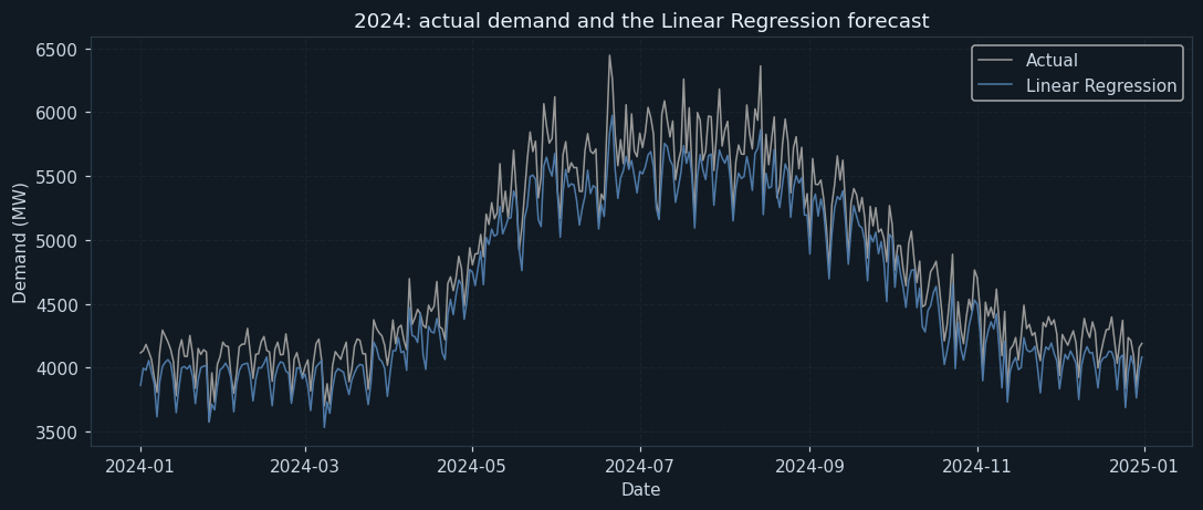
Actual demand through 2024 (grey) and Linear Regression's day-ahead forecast (blue).
The forecast follows the yearly cycle, the weekly dips and the summer peak closely. 2024 was never used for training, so this is how the model would have performed in real use.
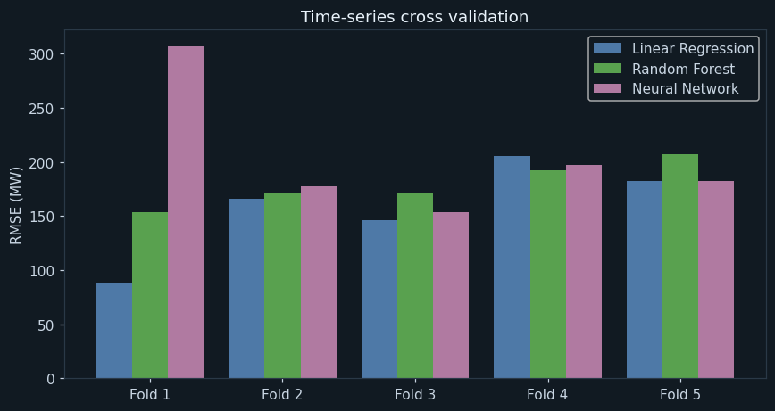
RMSE of each model in five time-series folds. Fold 1 trains on the first sixth of the data and tests on the next sixth; each later fold trains on more history.
Linear Regression has the lowest error in most folds. The neural network does badly in fold 1, when it has the least data to learn from, and only catches up later — neural networks need more data than simple models. The Random Forest gets worse in later folds because demand keeps growing beyond the range it was trained on, and a forest cannot predict values higher than any it has seen.
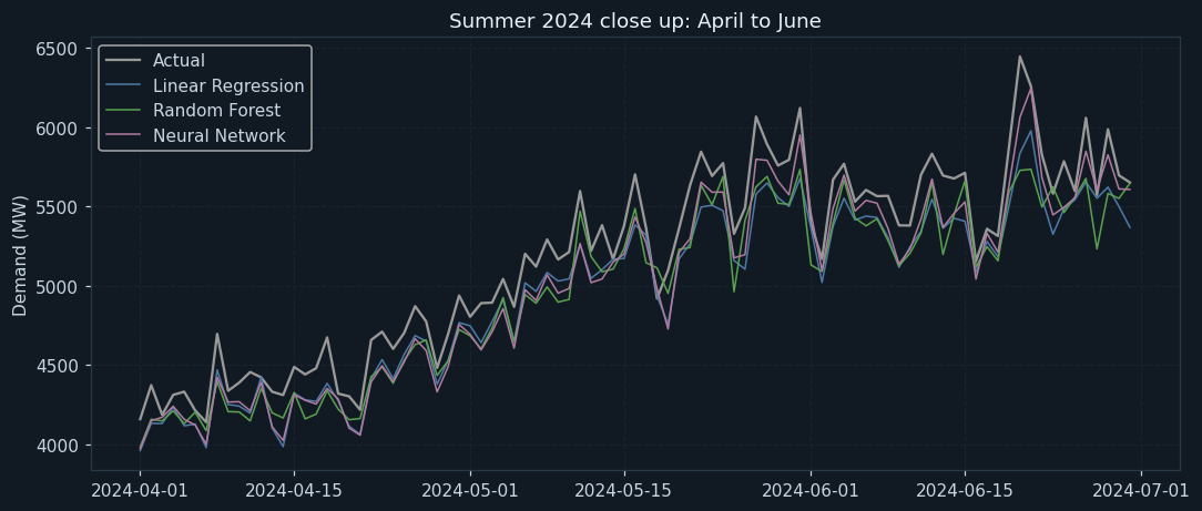
April to June 2024: actual demand and the three models' forecasts.
All three models follow the heat-driven rise. The differences between them are small next to the size of the summer swing — which is why the time-series cross validation, not one season's look, decided between them.
10Step 9 — Deployment
The chosen model is saved to demand_model.pkl. Each afternoon it would be given tomorrow's weather forecast, whether tomorrow is a weekend or holiday, and today's and last week's demand. For 1 January 2025, with a forecast maximum of 24 °C, it predicts 4008 MW MW.
In the control room the forecast would appear with its typical error beside it, so dispatchers schedule a margin above it — larger in summer, when chart 4 shows demand is most variable.
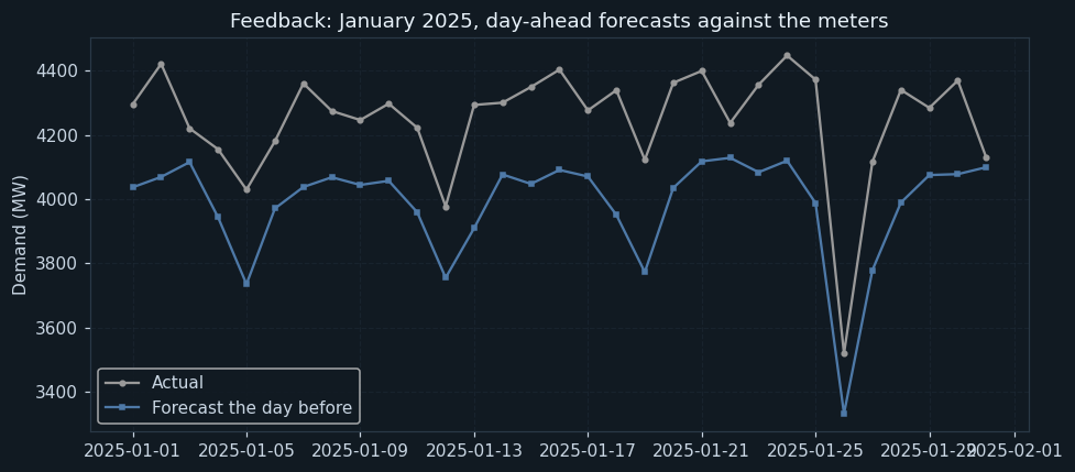
Each day of January 2025, forecast the evening before (blue) against the meters (grey).
The forecast follows the shape of the month — the Sunday dips and day-to-day movement — but the blue line sits below the grey one almost every day. The model was trained on 2022–2023 demand and the city has grown since. The Feedback step measures that gap.
11Step 10 — Feedback
Every day of January 2025 was forecast the evening before and compared with the meters. The RMSE was 276.7 MW, against 172.0 MW for January 2024 — well above the 25% tolerance the program allows, so it recommends retraining.
The cause is visible in chart 8 and in one number: the average error in January 2025 was 263.4 MW (actual minus forecast). The forecasts are consistently too low. Demand grows several per cent a year, as the engineer warned in the interviews; a model trained on 2022–2023 does not know the city is bigger now.
The fix is part of the methodology's loop: retrain regularly — every quarter — on the latest data, and consider a feature that captures growth, such as the number of connected consumers. Without the feedback step, the model would quietly under-forecast more each month, and the first sign would be load-shedding in the next summer.
12Ethical considerations
Under-forecasting leads to load-shedding, which usually falls on poorer areas first. An error is not only a number; the margin chosen above the forecast decides who goes without power.
Linear Regression was chosen partly because its coefficients can be explained. When a forecast goes wrong in a heatwave, the dispatchers need to understand why.
City-level demand reveals nothing personal, but household meter data does — when people are home, when they sleep. A finer-grained version must aggregate meter data before modelling.
Better forecasts let the grid rely more on solar and wind and less on fossil plants kept running as a safety margin — the SDG 13 side of the project.
13Source code
The whole program, laid out as the ten steps of the methodology. Every chart and number on this page came out of running it.
# ---------------------------------------------------------------------------
# power_demand.py
#
# Capstone project: forecasting tomorrow's peak electricity demand for a
# city, so the distribution company can buy and schedule the right amount
# of power - no blackouts, and no expensive power bought and wasted.
#
# CBSE Class XII, Artificial Intelligence (843), Part C - Capstone Project.
# SDG 7 (Affordable and Clean Energy) and SDG 13 (Climate Action).
#
# Data Science Methodology, 10 steps. REGRESSION on a time series. Three
# models are compared - Linear Regression, a Random Forest and a neural
# network (a multi-layer perceptron) - and, because this is a forecast,
# they are trained on the past and tested on a later year, then checked
# with time-series cross validation.
#
# Libraries: pandas, numpy, matplotlib, scikit-learn, joblib.
# ---------------------------------------------------------------------------

# %% Step 1 - Business Understanding
print("=" * 64)
print("TOMORROW'S ELECTRICITY DEMAND")
print("=" * 64)
print("Problem : power for tomorrow is bought today; a bad guess means")
print("          load-shedding or paying for power nobody uses")
print("Goal    : forecast tomorrow's peak demand (MW) from weather and calendar")
print()

# %% Step 2 - Analytic Approach
print("Analytic approach : predictive - regression on a time series")
print()

# %% Step 3 - Data Requirements
import pandas as pd
import numpy as np
import matplotlib.pyplot as plt
from sklearn.linear_model import LinearRegression
from sklearn.ensemble import RandomForestRegressor
from sklearn.neural_network import MLPRegressor
from sklearn.pipeline import make_pipeline
from sklearn.preprocessing import StandardScaler
from sklearn.model_selection import TimeSeriesSplit
from sklearn.metrics import mean_absolute_error, mean_squared_error, r2_score
import joblib

pd.set_option("display.width", 130)
pd.set_option("display.max_columns", 20)

# %% Step 4 - Data Collection
data = pd.read_csv("power_demand.csv", parse_dates=["date"])
print("Rows collected :", len(data))
print("Dates          :", data["date"].min().date(), "to", data["date"].max().date())
print(data.head(6))
print()

# %% Step 5 - Data Understanding
print("--- Step 5: Data Understanding ---")
print("Missing values:")
print(data.isnull().sum().to_string())
print("Days with demand recorded as 0 :", (data["demand_mw"] == 0).sum())
print()
print(data.describe().round(1))
print()

ok = data[data["demand_mw"] > 0]

# Chart 1: demand every day for three years.
plt.figure(figsize=(10, 4))
plt.plot(ok["date"], ok["demand_mw"], color="#f28e2b", linewidth=0.8)
plt.title("Daily peak demand, 2022-2024")
plt.xlabel("Date")
plt.ylabel("Demand (MW)")
plt.grid(True, linestyle="--", alpha=0.3)
plt.tight_layout()
plt.savefig("chart1_demand.png")
plt.close()

# Chart 2: temperature against demand.
plt.figure(figsize=(7, 5))
plt.scatter(ok["max_temp_c"], ok["demand_mw"], s=8, alpha=0.5, color="#e15759")
plt.title("Maximum temperature and demand")
plt.xlabel("Maximum temperature (deg C)")
plt.ylabel("Demand (MW)")
plt.grid(True, linestyle="--", alpha=0.3)
plt.tight_layout()
plt.savefig("chart2_temperature.png")
plt.close()

# Chart 3: average demand on each day of the week.
weekday = ok.groupby(ok["date"].dt.dayofweek)["demand_mw"].mean()
names = ["Mon", "Tue", "Wed", "Thu", "Fri", "Sat", "Sun"]
print("Average demand by day of the week (MW):")
for i in range(7):
    print("  " + names[i], round(weekday[i]))
print()
plt.figure(figsize=(7, 4))
plt.bar(names, weekday.values, color=["#4e79a7"] * 5 + ["#9c9c9c", "#9c9c9c"])
plt.ylim(weekday.min() - 300, weekday.max() + 100)
plt.title("Average demand by day of the week")
plt.ylabel("Demand (MW)")
plt.tight_layout()
plt.savefig("chart3_weekday.png")
plt.close()

# %% Step 6 - Data Preparation
print("--- Step 6: Data Preparation ---")
before = len(data)
data = data.drop_duplicates(subset="date").sort_values("date").reset_index(drop=True)
print("Duplicate dates removed        :", before - len(data))

# A demand of 0 is a grid failure, not a real demand: it becomes missing.
# Missing days are then filled by interpolating between the days either
# side, which suits a smooth day-to-day series.
data["demand_mw"] = pd.to_numeric(data["demand_mw"]).replace(0, np.nan)
gaps = data["demand_mw"].isnull().sum()
data["demand_mw"] = data["demand_mw"].interpolate()
print("Missing or zero days filled    :", gaps, "(interpolated)")

# Feature engineering - all from information known the day before.
data["day_of_week"] = data["date"].dt.dayofweek
data["is_sunday"] = (data["day_of_week"] == 6).astype(int)
data["is_saturday"] = (data["day_of_week"] == 5).astype(int)
data["month"] = data["date"].dt.month
data["cooling_degrees"] = np.maximum(0, data["max_temp_c"] - 27)       # heat above 27 drives ACs
data["demand_yesterday"] = data["demand_mw"].shift(1)
data["demand_last_week"] = data["demand_mw"].shift(7)
data = data.dropna().reset_index(drop=True)
features = ["max_temp_c", "cooling_degrees", "humidity_pct", "holiday", "is_saturday", "is_sunday",
            "month", "demand_yesterday", "demand_last_week"]
print("Rows after making lag features :", len(data), "(first 7 days have no 'last week')")
print("Features used                  :", features)
print()

# Chart 4: demand in each month, as box plots.
plt.figure(figsize=(9, 4.3))
plt.boxplot([data[data["month"] == m]["demand_mw"] for m in range(1, 13)],
            labels=["J", "F", "M", "A", "M", "J", "J", "A", "S", "O", "N", "D"])
plt.title("Demand in each month (2022-2024)")
plt.ylabel("Demand (MW)")
plt.grid(True, axis="y", linestyle="--", alpha=0.3)
plt.tight_layout()
plt.savefig("chart4_months.png")
plt.close()

# %% Step 7 - Modelling
print("--- Step 7: Modelling ---")
# A forecast must be tested on a future the model has not seen, so the
# rows are NOT shuffled: train on 2022-2023, test on 2024.
train = data[data["date"].dt.year <= 2023]
test = data[data["date"].dt.year == 2024]
X_train, y_train = train[features], train["demand_mw"]
X_test, y_test = test[features], test["demand_mw"]
print("Training days (2022-2023) :", len(train))
print("Testing days (2024)       :", len(test))
print()

models = {
    "Linear Regression": LinearRegression(),
    "Random Forest": RandomForestRegressor(n_estimators=300, min_samples_leaf=2, random_state=0),
    "Neural Network": make_pipeline(StandardScaler(),
                                    MLPRegressor(hidden_layer_sizes=(32, 16), max_iter=3000,
                                                 learning_rate_init=0.01, random_state=0)),
}
for name in models:
    models[name].fit(X_train, y_train)
print("Neural network layers : input 9 -> 32 -> 16 -> output 1")
print()

# %% Step 8 - Evaluation
print("--- Step 8: Evaluation ---")
average = y_test.mean()
predictions = {}
for name in models:
    pred = models[name].predict(X_test)
    predictions[name] = pred
    rmse = np.sqrt(mean_squared_error(y_test, pred))
    print(name)
    print("  " + name + " MAE  :", round(mean_absolute_error(y_test, pred), 1), "MW")
    print("  " + name + " RMSE :", round(rmse, 1), "MW")
    print("  " + name + " R2   :", round(r2_score(y_test, pred), 3))
    print("  " + name + " RMSE as % of average demand :", round(rmse / average * 100, 2), "%")
naive = test["demand_yesterday"]
print("Baseline 'same as yesterday' RMSE :", round(np.sqrt(mean_squared_error(y_test, naive)), 1), "MW")
print()

# Time-series cross validation: each fold trains on everything before it
# and tests on the block that follows - never on the past.
tscv = TimeSeriesSplit(n_splits=5)
cv_rmse = {name: [] for name in models}
X_all, y_all = data[features], data["demand_mw"]
for train_idx, test_idx in tscv.split(X_all):
    for name in models:
        m = {"Linear Regression": LinearRegression(),
             "Random Forest": RandomForestRegressor(n_estimators=300, min_samples_leaf=2, random_state=0),
             "Neural Network": make_pipeline(StandardScaler(),
                                             MLPRegressor(hidden_layer_sizes=(32, 16), max_iter=3000,
                                                          learning_rate_init=0.01, random_state=0))}[name]
        m.fit(X_all.iloc[train_idx], y_all.iloc[train_idx])
        p = m.predict(X_all.iloc[test_idx])
        cv_rmse[name].append(np.sqrt(mean_squared_error(y_all.iloc[test_idx], p)))
print("Time-series cross validation, RMSE (MW) in each fold:")
for name in models:
    print("  " + name.ljust(18), np.round(cv_rmse[name], 1), " mean", round(np.mean(cv_rmse[name]), 1))
print()

# Chart 5: actual and predicted demand through 2024.
plt.figure(figsize=(10, 4.3))
plt.plot(test["date"], y_test, color="#999999", linewidth=1, label="Actual")
plt.plot(test["date"], predictions["Linear Regression"], color="#4e79a7", linewidth=1, label="Linear Regression")
plt.title("2024: actual demand and the Linear Regression forecast")
plt.xlabel("Date")
plt.ylabel("Demand (MW)")
plt.legend()
plt.grid(True, linestyle="--", alpha=0.3)
plt.tight_layout()
plt.savefig("chart5_forecast_2024.png")
plt.close()

# Chart 6: error in each time-series fold for the three models.
x = np.arange(5)
plt.figure(figsize=(8, 4.3))
plt.bar(x - 0.27, cv_rmse["Linear Regression"], width=0.27, label="Linear Regression", color="#4e79a7")
plt.bar(x, cv_rmse["Random Forest"], width=0.27, label="Random Forest", color="#59a14f")
plt.bar(x + 0.27, cv_rmse["Neural Network"], width=0.27, label="Neural Network", color="#b07aa1")
plt.xticks(x, ["Fold 1", "Fold 2", "Fold 3", "Fold 4", "Fold 5"])
plt.ylabel("RMSE (MW)")
plt.title("Time-series cross validation")
plt.legend()
plt.tight_layout()
plt.savefig("chart6_tscv.png")
plt.close()

# Chart 7: what the linear model's coefficients mean, per unit.
coef = pd.Series(models["Linear Regression"].coef_, index=features)
print("Linear Regression coefficients:")
print(coef.round(2).to_string())
print()
summer = test[(test["date"].dt.month >= 4) & (test["date"].dt.month <= 6)]
plt.figure(figsize=(10, 4.3))
plt.plot(summer["date"], summer["demand_mw"], color="#999999", label="Actual")
for name, col in [["Linear Regression", "#4e79a7"], ["Random Forest", "#59a14f"], ["Neural Network", "#b07aa1"]]:
    plt.plot(summer["date"], models[name].predict(summer[features]), color=col, linewidth=1, label=name)
plt.title("Summer 2024 close up: April to June")
plt.ylabel("Demand (MW)")
plt.legend()
plt.grid(True, linestyle="--", alpha=0.3)
plt.tight_layout()
plt.savefig("chart7_summer.png")
plt.close()

# %% Step 9 - Deployment
print("--- Step 9: Deployment ---")
best = models["Linear Regression"]
joblib.dump(best, "demand_model.pkl")
model = joblib.load("demand_model.pkl")
last = data.iloc[-1]
last_week = data.iloc[-7]
tomorrow = pd.DataFrame({"max_temp_c": [24.0], "cooling_degrees": [0.0], "humidity_pct": [58], "holiday": [0],
                         "is_saturday": [0], "is_sunday": [0], "month": [1],
                         "demand_yesterday": [last["demand_mw"]], "demand_last_week": [last_week["demand_mw"]]})
print("Forecast for 1 January 2025 (24 deg C forecast) :", round(model.predict(tomorrow)[0]), "MW")
print()

# %% Step 10 - Feedback
print("--- Step 10: Feedback ---")
# Each day of January 2025 is forecast the evening before, then compared
# with what the meters actually recorded.
jan = pd.read_csv("january_2025.csv", parse_dates=["date"])
history = pd.concat([data[["date", "demand_mw"]], jan[["date", "demand_mw"]]]).reset_index(drop=True)
jan["day_of_week"] = jan["date"].dt.dayofweek
jan["is_sunday"] = (jan["day_of_week"] == 6).astype(int)
jan["is_saturday"] = (jan["day_of_week"] == 5).astype(int)
jan["month"] = 1
jan["cooling_degrees"] = np.maximum(0, jan["max_temp_c"] - 27)
jan["demand_yesterday"] = history["demand_mw"].shift(1).iloc[-len(jan):].values
jan["demand_last_week"] = history["demand_mw"].shift(7).iloc[-len(jan):].values
jan_pred = model.predict(jan[features])
jan_rmse = np.sqrt(mean_squared_error(jan["demand_mw"], jan_pred))
test_rmse = np.sqrt(mean_squared_error(y_test, predictions["Linear Regression"]))
jan_2024 = test[test["date"].dt.month == 1]
jan_2024_rmse = np.sqrt(mean_squared_error(jan_2024["demand_mw"], model.predict(jan_2024[features])))
print("Days forecast in January 2025     :", len(jan))
print("RMSE, January 2025                :", round(jan_rmse, 1), "MW")
print("RMSE, January 2024 (test year)    :", round(jan_2024_rmse, 1), "MW")
print("RMSE, all of 2024                 :", round(test_rmse, 1), "MW")
print("Average error in January 2025     :", round((jan["demand_mw"] - jan_pred).mean(), 1),
      "MW (actual minus forecast)")
if jan_rmse > 1.25 * jan_2024_rmse:
    print("Feedback: January 2025 errors are well above last January's - retrain.")
else:
    print("Feedback: January 2025 is in line with last January - keep the model, retrain each quarter.")

# Chart 8: January 2025, forecast against actual.
plt.figure(figsize=(9, 4))
plt.plot(jan["date"], jan["demand_mw"], marker="o", markersize=3, color="#999999", label="Actual")
plt.plot(jan["date"], jan_pred, marker="s", markersize=3, color="#4e79a7", label="Forecast the day before")
plt.title("Feedback: January 2025, day-ahead forecasts against the meters")
plt.ylabel("Demand (MW)")
plt.legend()
plt.grid(True, linestyle="--", alpha=0.3)
plt.tight_layout()
plt.savefig("chart8_january_2025.png")
plt.close()
The library calls it is built from
| Call | Step | What it does |
|---|---|---|
pd.read_csv(parse_dates=["date"]) | Step 4 | Reads the file with real dates |
drop_duplicates(subset="date") | Step 6 | One row per day |
replace(0, np.nan) / interpolate() | Step 6 | Treats a grid failure as missing and fills gaps |
dt.dayofweek / dt.month | Step 6 | Calendar features from the date |
shift(1) / shift(7) | Step 6 | Lag features: yesterday's and last week's demand |
np.maximum(0, temp - 27) | Step 6 | Cooling degrees above 27 °C |
LinearRegression / RandomForestRegressor / MLPRegressor | Step 7 | The three models |
make_pipeline(StandardScaler(), MLPRegressor(...)) | Step 7 | Scales the inputs for the neural network |
TimeSeriesSplit(n_splits=5) | Step 8 | Cross validation that never tests on the past |
mean_absolute_error / mean_squared_error / r2_score | Step 8 | The regression metrics |
joblib.dump() / load() | Step 9 | Saves and reloads the model |
14Output of a real run
================================================================
TOMORROW'S ELECTRICITY DEMAND
================================================================
Problem : power for tomorrow is bought today; a bad guess means
          load-shedding or paying for power nobody uses
Goal    : forecast tomorrow's peak demand (MW) from weather and calendar

Analytic approach : predictive - regression on a time series

Rows collected : 1097
Dates          : 2022-01-01 to 2024-12-31
        date  max_temp_c  humidity_pct  holiday  demand_mw
0 2022-01-01        23.0          50.0        0     3782.0
1 2022-01-02        23.4          71.0        0     3616.0
2 2022-01-03        22.4          73.0        0     3749.0
3 2022-01-04        21.4          43.0        0     3738.0
4 2022-01-05        22.1          57.0        0     3735.0
5 2022-01-06        21.2          75.0        0     3892.0

--- Step 5: Data Understanding ---
Missing values:
date            0
max_temp_c      0
humidity_pct    0
holiday         0
demand_mw       9
Days with demand recorded as 0 : 1

                                date  max_temp_c  humidity_pct  holiday  demand_mw
count                           1097      1097.0        1097.0   1097.0     1088.0
mean   2023-07-02 08:46:22.862351872        31.2          61.8      0.0     4581.8
min              2022-01-01 00:00:00        18.5          32.0      0.0        0.0
25%              2022-10-02 00:00:00        25.1          52.0      0.0     4008.8
50%              2023-07-02 00:00:00        31.1          59.0      0.0     4421.5
75%              2024-04-01 00:00:00        37.5          71.0      0.0     5183.2
max              2024-12-31 00:00:00        42.6          98.0      1.0     6445.0
std                              NaN         6.5          13.6      0.1      691.7

Average demand by day of the week (MW):
  Mon 4587
  Tue 4630
  Wed 4670
  Thu 4644
  Fri 4682
  Sat 4565
  Sun 4330

--- Step 6: Data Preparation ---
Duplicate dates removed        : 1
Missing or zero days filled    : 10 (interpolated)
Rows after making lag features : 1089 (first 7 days have no 'last week')
Features used                  : ['max_temp_c', 'cooling_degrees', 'humidity_pct', 'holiday', 'is_saturday', 'is_sunday', 'month', 'demand_yesterday', 'demand_last_week']

--- Step 7: Modelling ---
Training days (2022-2023) : 723
Testing days (2024)       : 366

Neural network layers : input 9 -> 32 -> 16 -> output 1

--- Step 8: Evaluation ---
Linear Regression
  Linear Regression MAE  : 190.6 MW
  Linear Regression RMSE : 213.5 MW
  Linear Regression R2   : 0.91
  Linear Regression RMSE as % of average demand : 4.45 %
Random Forest
  Random Forest MAE  : 185.0 MW
  Random Forest RMSE : 220.0 MW
  Random Forest R2   : 0.904
  Random Forest RMSE as % of average demand : 4.58 %
Neural Network
  Neural Network MAE  : 166.6 MW
  Neural Network RMSE : 186.7 MW
  Neural Network R2   : 0.931
  Neural Network RMSE as % of average demand : 3.89 %
Baseline 'same as yesterday' RMSE : 256.0 MW

Time-series cross validation, RMSE (MW) in each fold:
  Linear Regression  [ 88.6 166.1 146.5 205.4 182.4]  mean 157.8
  Random Forest      [153.5 170.7 171.  192.6 207. ]  mean 179.0
  Neural Network     [307.2 177.6 153.9 197.3 182.5]  mean 203.7

Linear Regression coefficients:
max_temp_c           -7.26
cooling_degrees      77.68
humidity_pct          2.24
holiday            -457.10
is_saturday        -115.66
is_sunday          -289.77
month                 6.80
demand_yesterday      0.34
demand_last_week      0.05

--- Step 9: Deployment ---
Forecast for 1 January 2025 (24 deg C forecast) : 4008 MW

--- Step 10: Feedback ---
Days forecast in January 2025     : 31
RMSE, January 2025                : 276.7 MW
RMSE, January 2024 (test year)    : 172.0 MW
RMSE, all of 2024                 : 213.5 MW
Average error in January 2025     : 263.4 MW (actual minus forecast)
Feedback: January 2025 errors are well above last January's - retrain.15The same project in Orange
The same forecast can be built in Orange; the Timeseries add-on helps with the date column and lag features. The tool is Orange Data Mining.
| Widget | What it does |
|---|---|
| File | Load power_demand.csv; set demand_mw as the target. |
| Select Rows + Impute | Treat 0 MW as missing; impute missing days. |
| Feature Constructor | Make cooling_degrees, is_sunday and the lag columns (or use the Timeseries add-on). |
| Line Plot / Scatter Plot | Draw demand over time and against temperature. |
| Linear Regression, Random Forest, Neural Network | The three learners. |
| Data Sampler (by date) + Test and Score | Train on 2022–2023 and test on 2024 — never use random cross validation for a forecast. |
16Testing
Every case was run: each gives the whole program a small input of its own.
| Test case | Expected | Actual | Result |
|---|---|---|---|
| Three years of days | Rows collected : 1097 | Rows collected : 1097 | Pass |
| One date entered twice is removed | Duplicate dates removed : 1 | Duplicate dates removed : 1 | Pass |
| Nine blank days and one grid failure (0) are filled | Missing or zero days filled : 10 (interpolated) | Missing or zero days filled : 10 (interpolated) | Pass |
| The model beats 'same as yesterday' | Baseline 'same as yesterday' RMSE : 256.0 MW | Baseline 'same as yesterday' RMSE : 256.0 MW | Pass |
| Feedback catches the forecasts running low in 2025 | Average error in January 2025 : 263.4 MW (actual minus forecast) | Average error in January 2025 : 263.4 MW (actual minus forecast) | Pass |
| Demand that is an exact rule of heat and Sunday: Linear Regression finds it | Linear Regression R2 : 1.0 | Linear Regression R2 : 1.0 | Pass |
| ...and learns 100 MW per degree above 27 | cooling_degrees 100.0 | cooling_degrees 100.0 | Pass |
| Three blank days in a row are interpolated, not dropped | Missing or zero days filled : 3 (interpolated) | Missing or zero days filled : 3 (interpolated) | Pass |
17Team roles and timeline
A capstone is done by a group of 3 to 5. A suggested split of the work, and a timeline across the year:
| Role | Responsible for |
|---|---|
| Project lead | Business understanding; interviews with dispatchers and engineers; presentation |
| Data lead | Demand, weather and holiday data; joining them by date |
| Analyst | Data understanding; cleaning; engineering the lag and heat features |
| Modeller | The three models, time-series cross validation, and the final choice |
| Documentation and video | Report, feedback analysis and the 3-minute video |
| When | Methodology steps | Deliverable |
|---|---|---|
| April – May | 1 Business Understanding, 2 Analytic Approach | Problem statement; interviews |
| June – July | 3 Data Requirements, 4 Data Collection | Three years of demand and weather joined |
| August | 5 Data Understanding, 6 Data Preparation | Clean series; engineered features |
| September – October | 7 Modelling, 8 Evaluation | Models compared with time-series CV |
| November | 9 Deployment, 10 Feedback | Day-ahead forecasts checked against a new month |
| December – January | Documentation and video | Report and 3-minute video |
18Results, limits and what next
- Every model beats 'same as yesterday'; Linear Regression's error on 2024 is 4.45 % of average demand.
- On one test year the neural network looked best, but time-series cross validation ranked Linear Regression first and showed the network was unstable with little data.
- Demand barely changes with temperature until about 27 °C, then rises steeply — air-conditioning.
- Sundays and holidays cut demand sharply; yesterday's demand carries strong momentum.
- In January 2025 the forecasts ran 263.4 MW (actual minus forecast) too low: the city had grown past the model.
Limitations
- Sample data for an imaginary city
- Uses actual temperatures where real use would have forecasts, which are less accurate
- No feature for the city's growth, so the model drifts as demand rises
- Daily peaks only — the grid also needs hour-by-hour forecasts
Future scope
- Retrain every quarter, and add a growth feature such as connected consumers
- Use weather forecasts rather than recorded temperatures
- Forecast hourly demand, and add rooftop solar generation
- Use real state demand from Grid-India for your capstone
What the team had to learn
- Why time-series data must be split by time, and TimeSeriesSplit
- Lag features with shift(), and what may and may not be used to forecast
- Multi-layer perceptrons (MLPRegressor) — the neural networks of Unit 6
- Why a model chosen on one test period can be the wrong choice
- Model drift, and why feedback is a step, not an afterthought
19Conclusion
The capstone built a day-ahead demand forecast that beats the 'same as yesterday' baseline and stays within the 5% of demand a dispatcher calls good. Feature engineering — heat above 27 °C, weekends, and yesterday's and last week's demand — did most of the work.
Choosing the model taught the most. A single test year favoured the neural network; time-series cross validation showed it was the least reliable, and Linear Regression the most. The handbook's validation techniques exist for exactly this reason.
The Feedback step found what every forecaster eventually meets: the world moves on. Within a month of 2025, the model was under-forecasting a growing city. Retraining on the latest data is not a repair but a permanent part of deploying a forecast.
20The 3-minute video script
Part C asks for a video of exactly three minutes with six parts. A script, timed to the second:
| Time | Part | What to say and show |
|---|---|---|
| 0:00 – 0:25 | a. Problem statement | Show a power-cut notice and a control room. "Power for tomorrow is bought today. Guess wrong and there is load-shedding, or wasted money." |
| 0:25 – 0:40 | b. SDG alignment | SDG 7 and 13 icons. "Reliable, affordable power — and a grid that can rely more on clean energy." |
| 0:40 – 1:15 | c. AI concepts and algorithms | "Predictive regression on a time series. We compared Linear Regression, a Random Forest and a neural network, tested on a year they never saw, with time-series cross validation." |
| 1:15 – 2:15 | d. How it works | Show chart 2 (the 27 °C bend), the lag features, chart 6 (cross validation) and the forecast for 1 January. Then chart 8: the January 2025 feedback, the forecasts running low. |
| 2:15 – 2:45 | e. Conclusion | "Our forecast is within about 4% of demand — but a growing city means it must be retrained every few months." |
| 2:45 – 3:00 | f. Acknowledgement | "We thank our AI teacher, [name], and the engineers who explained the grid to us." |
21Questions for the viva
▸Why didn't you shuffle the data before splitting it?
It is a time series. A forecast is always made for the future, so the model must be tested on days after the ones it learned from. Shuffling would let it learn from the future.
▸What is time-series cross validation?
Cross validation where each fold trains only on earlier data and tests on the block that follows, so the model is never tested on the past.
▸What are lag features, and why may you use them?
Values from earlier days, like yesterday's demand. They are known the day before the forecast, so using them is allowed; tomorrow's demand is not.
▸Why did you create the cooling_degrees feature?
Demand hardly changes below 27 °C and rises steeply above it, as air-conditioners switch on. The feature lets a linear model capture that bend.
▸The neural network was best on 2024. Why didn't you choose it?
Time-series cross validation showed it was the least reliable, especially with little data. Linear Regression had the lowest average error and can be explained.
▸Why can't a Random Forest forecast a growing city well?
A tree's prediction is an average of training values, so it can never predict higher than anything it has seen. As demand grows, it falls behind.
▸What did the Feedback step find?
In January 2025 the forecasts were too low by about 260 MW on average, because demand had grown since the training years. The model needs regular retraining.
▸Which SDGs does it align to?
SDG 7, Affordable and Clean Energy, and SDG 13, Climate Action.
22References
- Grid Controller of India (Grid-India) — daily power supply position reports — https://grid-india.in/
- Central Electricity Authority — load generation balance reports — https://cea.nic.in/
- India Meteorological Department — https://mausam.imd.gov.in/
- Hyndman, R. J. and Athanasopoulos, G. Forecasting: Principles and Practice (3rd ed.) — on time-series cross validation — https://otexts.com/fpp3/
- scikit-learn: TimeSeriesSplit, MLPRegressor — https://scikit-learn.org/stable/
- CBSE, Artificial Intelligence (Subject Code 843), Class XII curriculum, 2026-27 — Part C
- CBSE, Artificial Intelligence Student Handbook, Class XII — Unit 2, Data Science Methodology
- Rollins, J. B. (2015). Foundational Methodology for Data Science. IBM Analytics.
- scikit-learn — https://scikit-learn.org/stable/; pandas, NumPy and Matplotlib documentation
- LambdaLab — https://www.lambdalab.in