Reading Handwritten PIN Codes
Computer vision and a neural network on real handwriting: a multi-layer perceptron learns to read digits, OpenCV cuts PIN codes off envelope images — and the feedback step shows why 98% per digit is not 98% per letter.
1Introduction
India's six-digit PIN code, in use since 1972, tells the postal system where every letter is going. At a sorting centre, millions of envelopes must be read and routed every day — and on many of them, the PIN code is handwritten.
Reading handwriting by hand is slow and tiring, and a tired person misreads a 1 as a 7. Printed addresses can be read by machines easily; handwriting is the hard part.
This capstone builds a model that reads handwritten digits — on real handwriting, from a public dataset — and then uses OpenCV, as Unit 3 of the curriculum describes, to read whole PIN codes off envelope images. Following the Data Science Methodology to the end, it discovers that a model which reads single digits superbly still misreads a worrying share of whole PIN codes.
Industry, Innovation and Infrastructure
SDG 9 asks for resilient infrastructure and wider access to it. The postal network is infrastructure that reaches every village in India — it carries pensions, documents, medicines and online orders. Sorting mail by machine, by reading the handwritten PIN code, makes that network faster and cheaper, which matters most to the people far from any other service.
2Step 1 — Business Understanding
What is the problem that you are trying to solve? The handbook uses the 5W1H Problem Canvas for this step.
- • Staff at mail sorting centres
- • Everyone who sends or receives post, especially in remote areas
- • Handwritten PIN codes are slow to read by hand
- • Misread codes send letters to the wrong place and delay them for days
- • Mail sorting centres and courier hubs
- • Every day, as millions of envelopes pass through sorting machines
- • Faster, cheaper, more reliable post
- • Fewer letters lost or delayed
- • Learn to recognise each handwritten digit from labelled examples
- • Cut the PIN code into digits with OpenCV and read each one
Problem statement
Who would use it: Mail sorting centres of the postal service and courier companies, where envelopes and parcels are sorted by PIN code.
Talking to the stakeholders
The handbook pairs the 5W1H canvas with Design Thinking, which begins by empathising with the people who have the problem. The questions asked, and what each answer changed:
| Question asked | What we learned, and what it changed |
|---|---|
| To a sorting-centre supervisor: which envelopes cause the most trouble? | Handwritten ones; printed labels are already read by machine. That focused the project on handwritten digits only. |
| To the same supervisor: which digits are most often misread? | 1 and 7, 3 and 8, 4 and 9. That told us to look at which pairs the model confuses, not just its overall accuracy. |
| To a postal clerk: what happens when a PIN is misread? | The letter goes to the wrong district and comes back days later. One wrong digit spoils the whole PIN — which became the measure checked in the Feedback step. |
| To an engineer: how does the machine see an envelope? | A camera captures the address area; the PIN is cut out and each digit is separated. That defined the deployment pipeline: load, cut, resize, read. |
| To the supervisor: would a machine that is sometimes wrong be useful? | Yes, if it can pass the envelopes it is unsure about to a person. So the model's role is to sort most mail, not all of it. |
How it is handled today
Flexible and good with odd handwriting, but slow, and errors rise as people tire.
Easily read by machines (OCR), but only part of the mail has them.
Large postal systems use advanced recognition. This project shows, at small scale, how such a system is built and where it struggles.
Objectives
- To frame handwritten PIN reading with the 5W1H canvas
- To collect and understand a real dataset of labelled handwritten digits
- To prepare the images for a neural network
- To train a neural network (multi-layer perceptron) and compare it with Logistic Regression, using stratified 5-fold cross validation
- To read whole PIN codes from envelope images with OpenCV — loading, cutting and resizing them
- To measure, as feedback, how often whole PIN codes are read correctly
3Step 2 — Analytic Approach
Each image must be assigned one of ten classes — the digits 0 to 9 — so this is predictive analytics with multi-class classification, in the Computer Vision domain.
The model reads digits; turning ten digit predictions into a decision about an envelope (sort it, or send it to a person) is the prescriptive step that deployment adds.
| Candidate | Why it was considered |
|---|---|
| Neural network (MLP Classifier) | A multi-layer perceptron — Unit 6 of the curriculum — with 64 inputs (one per pixel), a hidden layer of 64 neurons and 10 outputs. It learns which pixel patterns make each digit. |
| Logistic Regression | A simpler baseline: one weighted sum per digit. If the neural network cannot beat it, the extra complexity is not worth it. |
| Rules by hand (rejected) | "A 1 is a vertical stroke" fails on real handwriting at once; there are too many ways to write each digit. Learning from examples is the only practical approach. |
4Step 3 — Data Requirements
A classification model needs many images of each digit, each labelled with the digit it shows, written by many different people so that the model learns handwriting in general rather than one person's style. The images must all be the same size, so each becomes a fixed list of numbers.
For deployment, envelope images are needed too, together with the true PIN, so that the whole pipeline can be checked end to end.
| Data needed | Type | Format | Source |
|---|---|---|---|
| Handwritten digit images | Unstructured (images), stored as numbers | 8 × 8 pixels, values 0–16 | UCI Optical Recognition of Handwritten Digits dataset |
| Digit label | Categorical | 0–9 | Same dataset |
| Envelope PIN images | Unstructured (images) | PNG, one six-digit PIN per image | Built from held-out digits of the same dataset |
| True PIN for each envelope | Text | Six digits | Recorded when the images were made |
5Step 4 — Data Collection
This project uses real data: the UCI "Optical Recognition of Handwritten Digits" dataset (Alpaydin and Kaynak, 1998), which ships with scikit-learn as load_digits(). It holds 1,797 digits written by 43 people, each scanned and reduced to an 8 × 8 grid of values from 0 (white) to 16 (black). It is secondary data, freely available, and credited in the references.
The first 1700 digits are saved to digits.csv for training and testing. The last 97 are never used for either: they are assembled into ten six-digit PIN-code images — "envelopes arriving at the sorting centre" — drawn large, as a scanner would capture them. Four of the ten are slightly rotated and smudged, as real envelopes are. Their true PINs are in pin_truth.csv.
| Column | Type | What it holds | Role |
|---|---|---|---|
image_id | text | An ID for the image | not used |
px0 … px63 | integer 0–16 | The 64 pixels of the 8 × 8 image, row by row | features |
digit | integer 0–9 | The digit the image shows | target |
digits.csv — Real handwritten digits: 64 pixel values and the digit, one row per image. 1,700 rows, 254.7 KB. Download the file
pin_codes — Ten envelope images, each a handwritten six-digit PIN code. 10 images, 129.7 KB.
pin_truth.csv — The true PIN of each envelope image. 10 rows, 0.2 KB. Download the file
The first four rows of digits.csv (pixel columns px9 to px62 not shown)
| image_id | px0 | px1 | px2 | px3 | px4 | px5 | px6 | px7 | … | digit |
|---|---|---|---|---|---|---|---|---|---|---|
D0001 | 0 | 0 | 5 | 13 | 9 | 1 | 0 | 0 | … | 0 |
D0002 | 0 | 0 | 0 | 12 | 13 | 5 | 0 | 0 | … | 1 |
D0003 | 0 | 0 | 0 | 4 | 15 | 12 | 0 | 0 | … | 2 |
D0004 | 0 | 0 | 7 | 15 | 13 | 1 | 0 | 0 | … | 3 |
pin_truth.csv
| file | true_pin |
|---|---|
pin_01.png | 497836 |
pin_02.png | 360384 |
pin_03.png | 780895 |
pin_04.png | 291897 |
pin_05.png | 621642 |
pin_06.png | 577288 |
pin_07.png | 221148 |
pin_08.png | 525836 |
pin_09.png | 344982 |
pin_10.png | 601915 |
6Step 5 — Data Understanding
Is the data collected representative of the problem to be solved?
The data is checked for completeness and balance: no missing values, and about 170 images of each digit, so no digit is under-represented. The pixel values run from 0 to 16, as the dataset documents.
Chart 1 shows what the computer receives — sixteen tiny 8 × 8 images, each just 64 numbers. Even at this resolution most are readable by eye. Chart 2 averages every image of each digit: the average 0 is a clear ring and the average 1 a clear stroke, which suggests the digits are separable. The averages of 3, 5, 8 and 9 overlap a good deal, hinting at where mistakes will be.
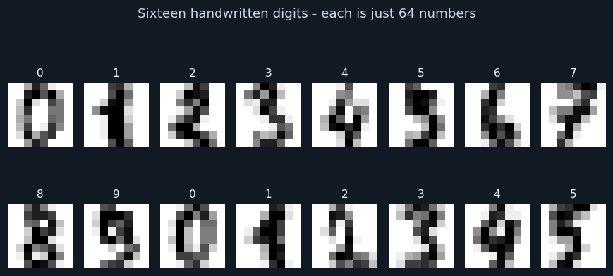
Sixteen images from the dataset, with their labels. Each is drawn from its 64 numbers.
At 8 × 8 pixels the digits are blocky but mostly recognisable. Every image is stored as 64 numbers from 0 to 16 — that is all the model ever sees.
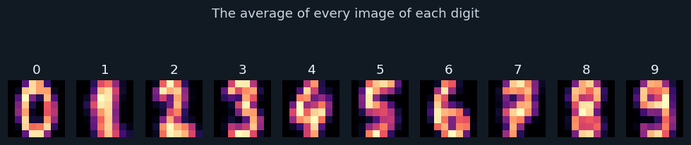
Each panel is the average of every image of one digit; brighter means the pixel is dark in most of them.
0, 1, 6 and 7 have distinct average shapes. 3, 5, 8 and 9 share curves in the same places, so they are the digits most likely to be confused.
7Step 6 — Data Preparation
Checked by comparing all 64 pixels and the label. None were found in the real data; the testing section shows the check working when duplicates are added deliberately.
Every pixel is divided by 16, giving values from 0 to 1. Neural networks learn faster and more reliably when inputs are on a small, similar scale.
Handled at deployment, not here: OpenCV resizes each digit cut from an envelope down to 8 × 8, and the values are put on the same 0–1 scale as the training data.
Feature engineering
Each 8 × 8 image is flattened into 64 features, one per pixel, read row by row. The model does not know that px0 and px1 are neighbours — it learns which combinations of pixels matter. (A Convolutional Neural Network, also in Unit 6, would use the 2-D layout directly; it is listed under future scope.)
No other features are engineered. The point of a neural network is that it learns its own internal features — in its hidden layer — from the raw pixels.
8Step 7 — Modelling
Every image is labelled with its digit, so this is supervised learning; with ten classes it is multi-class classification. The neural network makes it deep learning in the curriculum's sense — an artificial neural network.
The split is stratified: 1360 Testing images : 340 images for training and 340 for testing, each with the same share of every digit.
How the models work
The neural network has three layers. The input layer has 64 neurons, one per pixel. The hidden layer has 64 neurons; each computes a weighted sum of all 64 pixels plus a bias, and passes it through an activation function (ReLU). The output layer has 10 neurons, one per digit, and the digit whose neuron is strongest is the prediction. In all, the network has 4810 weights and biases.
Training adjusts all those weights to reduce the loss, pass after pass, using backpropagation — the error at the output is sent back through the network to update each weight a little (chart 3).
Logistic Regression, the baseline, learns one weighted sum of the 64 pixels for each digit, with no hidden layer.
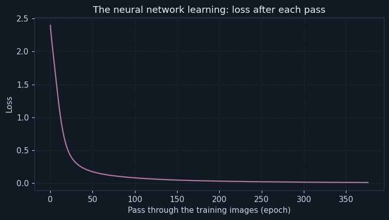
The network's loss — how wrong its predictions are on the training images — after each pass (epoch).
The loss falls steeply at first and then levels off: the network learns most of what it can in the first passes, and later passes fine-tune it. A loss curve that kept falling would suggest more training; one that rose would signal a problem.
9Step 8 — Evaluation
On the 340 test images, Logistic Regression scored an accuracy of 0.9706 and the neural network 0.9794. Stratified 5-fold cross validation confirms it: mean accuracy 0.9694 against 0.9812, with the network ahead in every fold.
For a ten-class problem, recall is reported for each digit, and the confusion matrix shows which digits are mistaken for which. The mistakes are few and scattered, and the misread images (chart 5) are mostly ones a person would find ambiguous.
The neural network is chosen. But single-digit accuracy is not the measure a sorting centre cares about — that is a whole PIN code read correctly, which is what the Feedback step tests.
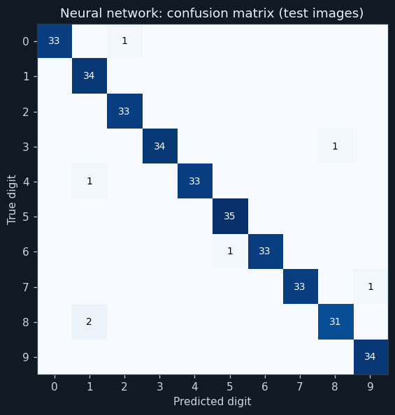
Rows are the true digits, columns the predictions, for the 340 test images. The diagonal holds correct predictions; every number off it is a mistake.
Almost everything is on the diagonal. The few mistakes are scattered, with an 8 read as a 1 the most common — two cases. A 10 × 10 matrix shows which digits are confused with which, which a single accuracy figure cannot.

Every test image the network misread, labelled true → predicted.
Most of these would make a person hesitate too: a thin 8 that looks like a 1, a 7 with a loop. Looking at the mistakes shows they are not random failures but genuinely ambiguous handwriting.
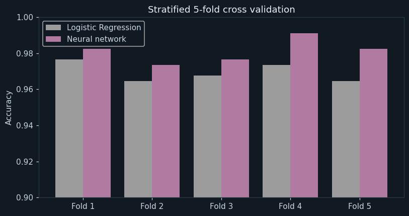
Accuracy of each model in each of the five folds. The axis starts at 0.9 to show the differences.
The neural network is ahead in every fold. Both are very accurate on single digits — the differences are about one percentage point — and the result does not depend on the split.
10Step 9 — Deployment
The network is saved to digit_model.pkl. Then the program does what a sorting machine would, using OpenCV — the library the curriculum introduces for loading, displaying and resizing images. For each envelope image it calls cv2.imread() to load it in grayscale, inverts it so the ink is bright as in the training data, cuts it into six equal parts, shrinks each to 8 × 8 with cv2.resize(), rescales the values to match the training data, and asks the network for each digit.
The program also checks that every image was actually loaded: cv2.imread() returns None, rather than raising an error, if a file is missing — a trap the testing section caught.
In a real sorting centre, an envelope whose digits are all read with high confidence would be routed automatically; any envelope with a doubtful digit would go to a person.
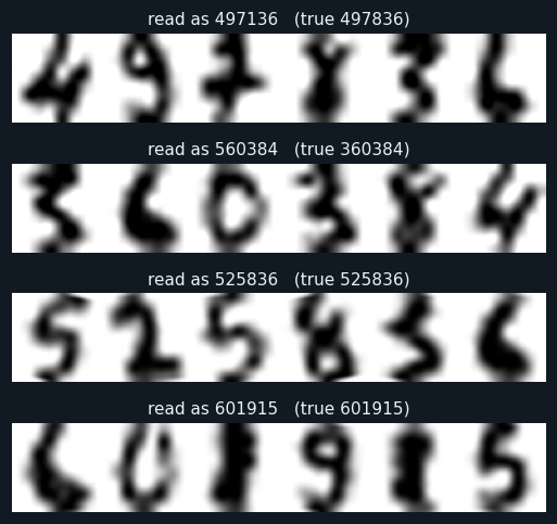
Four of the ten envelope images, with the PIN the model read and the true PIN.
OpenCV loaded each image, cut it into six digits and resized each to 8 × 8, and the network read them. The top envelope shows the kind of error that matters: one digit wrong, so the whole PIN is wrong.
11Step 10 — Feedback
The envelopes are the feedback: real handwriting the model never trained or tested on, passed through the whole pipeline. It read 56 of 60 digits correctly — and 6 of 10 whole PIN codes.
Two lessons come out of that. First, accuracy fell from about 98% on the test images to about 93% on the envelopes. The envelope digits went through a path the training images never did — enlarged, sometimes rotated and blurred, then shrunk again by OpenCV — so they look slightly different. A model is only as good as the match between the data it learned from and the data it meets.
Second, errors compound. A PIN is right only if all six digits are right; at 93.3% per digit, that happens only about two times in three. A sorting centre needs per-digit accuracy far above 99% — or the envelopes the model is unsure about sent to a person. That changes the project's requirement, and sends the methodology back to Data Requirements: train on digits that have been through the same scanning path.
With only ten envelopes, the split between clean and messy envelopes (3 of 6 clean, 3 of 4 messy) is too small to draw conclusions from — itself a feedback finding: more envelopes are needed before the system is trusted.
12Ethical considerations
A misread PIN delays a letter by days. For a pension, an exam admit card or medicine sent by post, that delay can do real harm. Sending doubtful envelopes to a person is the safeguard.
The dataset was written by 43 people. Handwriting styles differ between regions, age groups and scripts; a model trained on a narrow sample may serve some people's mail worse. Real systems must be trained and tested on handwriting from everyone they serve.
Automation changes the work at sorting centres. The interviews suggested people move to handling the hard cases rather than disappearing — but the effect on workers should be part of the discussion.
Envelopes carry names and addresses. A system should read only the PIN area and keep no images longer than needed.
13Source code
The whole program, laid out as the ten steps of the methodology. Every chart and number on this page came out of running it.
# ---------------------------------------------------------------------------
# pin_reader.py
#
# Capstone project: reading handwritten PIN codes on envelopes, so that
# letters and parcels can be sorted by machine.
#
# CBSE Class XII, Artificial Intelligence (843), Part C - Capstone Project.
# SDG 9 (Industry, Innovation and Infrastructure).
#
# Data Science Methodology, 10 steps. COMPUTER VISION with a NEURAL
# NETWORK. The data is real: the UCI handwritten digits dataset (8 x 8
# images). A multi-layer perceptron is compared with Logistic Regression,
# with stratified 5-fold cross validation; then OpenCV loads, splits and
# resizes whole PIN-code images for the model to read.
#
# Libraries: pandas, numpy, matplotlib, scikit-learn, OpenCV (cv2), joblib.
# ---------------------------------------------------------------------------

# %% Step 1 - Business Understanding
print("=" * 64)
print("READING HANDWRITTEN PIN CODES")
print("=" * 64)
print("Problem : millions of envelopes carry handwritten PIN codes;")
print("          reading them by hand is slow and error-prone")
print("Goal    : recognise each handwritten digit, and so the whole PIN")
print()

# %% Step 2 - Analytic Approach
print("Analytic approach : predictive - classification into 10 classes (0-9)")
print()

# %% Step 3 - Data Requirements
import os
import pandas as pd
import numpy as np
import matplotlib.pyplot as plt
import cv2
from sklearn.model_selection import train_test_split, StratifiedKFold, cross_val_score
from sklearn.linear_model import LogisticRegression
from sklearn.neural_network import MLPClassifier
from sklearn.metrics import accuracy_score, confusion_matrix, recall_score
import joblib

# %% Step 4 - Data Collection
data = pd.read_csv("digits.csv")
pixels = ["px" + str(i) for i in range(64)]
print("Images collected :", len(data))
print("Values per image :", len(pixels), "(an 8 x 8 grid)")
print("Pixel values run from", data[pixels].values.min(), "to", data[pixels].values.max())
print()

# %% Step 5 - Data Understanding
print("--- Step 5: Data Understanding ---")
print("Missing values in the whole table :", int(data.isnull().sum().sum()))
counts = data["digit"].value_counts().sort_index()
print("Images of each digit:")
print(counts.to_string())
print()

# Chart 1: sixteen of the images, as the computer stores them.
plt.figure(figsize=(8, 4.2))
for i in range(16):
    plt.subplot(2, 8, i + 1)
    plt.imshow(data.loc[i, pixels].values.astype(float).reshape(8, 8), cmap="gray_r")
    plt.title(str(data.loc[i, "digit"]), fontsize=10)
    plt.axis("off")
plt.suptitle("Sixteen handwritten digits - each is just 64 numbers")
plt.tight_layout()
plt.savefig("chart1_samples.png")
plt.close()

# Chart 2: the average image of each digit.
plt.figure(figsize=(9, 2.4))
for d in range(10):
    plt.subplot(1, 10, d + 1)
    plt.imshow(data[data["digit"] == d][pixels].mean().values.reshape(8, 8), cmap="magma")
    plt.title(str(d))
    plt.axis("off")
plt.suptitle("The average of every image of each digit")
plt.tight_layout()
plt.savefig("chart2_average_digits.png")
plt.close()

# %% Step 6 - Data Preparation
print("--- Step 6: Data Preparation ---")
before = len(data)
data = data.drop_duplicates(subset=pixels + ["digit"])
print("Duplicate images removed :", before - len(data))
# The pixel values run 0-16. Dividing by 16 puts them on a 0-1 scale,
# which helps a neural network learn.
X = data[pixels] / 16.0
y = data["digit"]
print("Pixels rescaled from 0-16 to 0-1")
print()

# %% Step 7 - Modelling
print("--- Step 7: Modelling ---")
X_train, X_test, y_train, y_test = train_test_split(X, y, test_size=0.2, stratify=y, random_state=3)
print("Training images :", len(X_train), " Testing images :", len(X_test))
logistic = LogisticRegression(max_iter=2000)
network = MLPClassifier(hidden_layer_sizes=(64,), max_iter=1000, random_state=0)
logistic.fit(X_train, y_train)
network.fit(X_train, y_train)
print("Neural network : 64 inputs -> 64 hidden neurons -> 10 outputs")
print("Weights learned by the network :", sum(w.size for w in network.coefs_) + sum(b.size for b in network.intercepts_))
print()

# Chart 3: the network's training - its loss falling with each pass.
plt.figure(figsize=(7, 4))
plt.plot(network.loss_curve_, color="#b07aa1")
plt.title("The neural network learning: loss after each pass")
plt.xlabel("Pass through the training images (epoch)")
plt.ylabel("Loss")
plt.grid(True, linestyle="--", alpha=0.4)
plt.tight_layout()
plt.savefig("chart3_loss_curve.png")
plt.close()

# %% Step 8 - Evaluation
print("--- Step 8: Evaluation ---")
pred_log = logistic.predict(X_test)
pred_net = network.predict(X_test)
print("Accuracy, Logistic Regression :", round(accuracy_score(y_test, pred_log), 4))
print("Accuracy, neural network      :", round(accuracy_score(y_test, pred_net), 4))
folds = StratifiedKFold(n_splits=5, shuffle=True, random_state=1)
cv_log = cross_val_score(LogisticRegression(max_iter=2000), X, y, cv=folds)
cv_net = cross_val_score(MLPClassifier(hidden_layer_sizes=(64,), max_iter=1000, random_state=0), X, y, cv=folds)
print("Accuracy in each fold, Logistic Regression :", np.round(cv_log, 3))
print("Accuracy in each fold, neural network      :", np.round(cv_net, 3))
print("Mean CV accuracy, Logistic Regression :", round(cv_log.mean(), 4))
print("Mean CV accuracy, neural network      :", round(cv_net.mean(), 4))
print()

cm = confusion_matrix(y_test, pred_net)
recall_each = recall_score(y_test, pred_net, average=None)
print("Recall for each digit (neural network):")
for d in range(10):
    print("  digit", d, ":", round(recall_each[d], 3))
pairs = []
for a in range(10):
    for b in range(10):
        if a != b and cm[a, b] > 0:
            pairs.append([cm[a, b], a, b])
pairs.sort(reverse=True)
print("Most common mistakes (true -> predicted, count):")
for count, a, b in pairs[:4]:
    print("  ", a, "->", b, ":", count)
print()

# Chart 4: the 10 x 10 confusion matrix.
plt.figure(figsize=(6.5, 5.5))
plt.imshow(cm, cmap="Blues")
for a in range(10):
    for b in range(10):
        if cm[a, b] > 0:
            plt.text(b, a, cm[a, b], ha="center", va="center", fontsize=9,
                     color="white" if cm[a, b] > cm.max() / 2 else "black")
plt.xticks(range(10))
plt.yticks(range(10))
plt.xlabel("Predicted digit")
plt.ylabel("True digit")
plt.title("Neural network: confusion matrix (test images)")
plt.tight_layout()
plt.savefig("chart4_confusion.png")
plt.close()

# Chart 5: the test images the network got wrong.
wrong = np.where(pred_net != y_test.values)[0]
plt.figure(figsize=(1.3 * max(len(wrong), 1) + 0.5, 2.0))
for k, i in enumerate(wrong):
    plt.subplot(1, len(wrong), k + 1)
    plt.imshow(X_test.iloc[i].values.reshape(8, 8), cmap="gray_r")
    plt.title(str(y_test.iloc[i]) + " -> " + str(pred_net[i]), fontsize=9)
    plt.axis("off")
plt.tight_layout()
plt.savefig("chart5_mistakes.png")
plt.close()

# Chart 6: accuracy in each fold, both models.
x = np.arange(5)
plt.figure(figsize=(7.5, 4))
plt.bar(x - 0.2, cv_log, width=0.4, label="Logistic Regression", color="#9c9c9c")
plt.bar(x + 0.2, cv_net, width=0.4, label="Neural network", color="#b07aa1")
plt.xticks(x, ["Fold 1", "Fold 2", "Fold 3", "Fold 4", "Fold 5"])
plt.ylim(0.9, 1.0)
plt.ylabel("Accuracy")
plt.title("Stratified 5-fold cross validation")
plt.legend()
plt.tight_layout()
plt.savefig("chart6_kfold.png")
plt.close()

# %% Step 9 - Deployment
print("--- Step 9: Deployment ---")
joblib.dump(network, "digit_model.pkl")
model = joblib.load("digit_model.pkl")
truth = pd.read_csv("pin_truth.csv", dtype={"true_pin": str})
results = []
for k in range(len(truth)):
    name = truth.loc[k, "file"]
    strip = cv2.imread(os.path.join("pin_codes", name), cv2.IMREAD_GRAYSCALE)   # load with OpenCV
    if strip is None:                         # imread gives None, not an error, if the file is missing
        raise FileNotFoundError("Could not read pin_codes/" + name)
    strip = 255 - strip                                                          # ink becomes bright
    read = ""
    for j in range(6):
        digit_img = strip[:, j * 64:(j + 1) * 64]                                 # cut out one digit
        small = cv2.resize(digit_img, (8, 8), interpolation=cv2.INTER_AREA)       # resize to 8 x 8
        vector = (small / 255.0 * 16).round() / 16.0                              # same 0-1 scale as training
        read = read + str(model.predict(vector.reshape(1, 64))[0])
    results.append([name, truth.loc[k, "true_pin"], read])
    status = "correct" if read == truth.loc[k, "true_pin"] else "WRONG"
    print(name, " true", truth.loc[k, "true_pin"], " read", read, " ", status)
print()

# Chart 7: four of the PIN images, with what the model read.
plt.figure(figsize=(9, 4.5))
for n, k in enumerate([0, 1, 7, 9]):
    img = cv2.imread(os.path.join("pin_codes", results[k][0]), cv2.IMREAD_GRAYSCALE)
    plt.subplot(4, 1, n + 1)
    plt.imshow(img, cmap="gray")
    plt.title("read as " + results[k][2] + "   (true " + results[k][1] + ")", fontsize=10)
    plt.axis("off")
plt.tight_layout()
plt.savefig("chart7_pin_codes.png")
plt.close()

# %% Step 10 - Feedback
print("--- Step 10: Feedback ---")
digits_right = 0
pins_right = 0
clean_right = 0
messy_right = 0
for k in range(len(results)):
    true_pin, read = results[k][1], results[k][2]
    digits_right = digits_right + sum(1 for a, b in zip(true_pin, read) if a == b)
    if true_pin == read:
        pins_right = pins_right + 1
        if k < 6:
            clean_right = clean_right + 1
        else:
            messy_right = messy_right + 1
print("Digits read correctly on envelopes :", digits_right, "of", 6 * len(results))
print("Whole PIN codes read correctly     :", pins_right, "of", len(results))
print("Clean envelopes, PINs correct      :", clean_right, "of 6")
print("Messy envelopes, PINs correct      :", messy_right, "of 4")
per_digit = digits_right / (6 * len(results))
print("If each digit is right with probability", round(per_digit, 3), ", a 6-digit PIN is all right")
print("with probability about", round(per_digit ** 6, 3))
The library calls it is built from
| Call | Step | What it does |
|---|---|---|
pd.read_csv() | Step 4 | Reads the 1,700 labelled digits |
values.reshape(8, 8) + plt.imshow() | Step 5 | Turns 64 numbers back into an image to look at |
drop_duplicates(subset=pixels + ["digit"]) | Step 6 | Finds images repeated pixel for pixel |
X / 16.0 | Step 6 | Rescales pixels from 0–16 to 0–1 |
MLPClassifier(hidden_layer_sizes=(64,)) | Step 7 | The neural network |
network.loss_curve_ | Step 7 | The loss after each training pass |
confusion_matrix() / recall_score(average=None) | Step 8 | The 10 × 10 matrix and recall per digit |
StratifiedKFold + cross_val_score() | Step 8 | Stratified 5-fold cross validation |
cv2.imread(..., cv2.IMREAD_GRAYSCALE) | Step 9 | OpenCV loads an envelope image |
cv2.resize(..., (8, 8), interpolation=cv2.INTER_AREA) | Step 9 | OpenCV shrinks each digit to the training size |
joblib.dump() / load() | Step 9 | Saves and reloads the network |
14Output of a real run
================================================================
READING HANDWRITTEN PIN CODES
================================================================
Problem : millions of envelopes carry handwritten PIN codes;
          reading them by hand is slow and error-prone
Goal    : recognise each handwritten digit, and so the whole PIN

Analytic approach : predictive - classification into 10 classes (0-9)

Images collected : 1700
Values per image : 64 (an 8 x 8 grid)
Pixel values run from 0 to 16

--- Step 5: Data Understanding ---
Missing values in the whole table : 0
Images of each digit:
digit
0    169
1    172
2    167
3    173
4    171
5    173
6    171
7    169
8    164
9    171

--- Step 6: Data Preparation ---
Duplicate images removed : 0
Pixels rescaled from 0-16 to 0-1

--- Step 7: Modelling ---
Training images : 1360  Testing images : 340
Neural network : 64 inputs -> 64 hidden neurons -> 10 outputs
Weights learned by the network : 4810

--- Step 8: Evaluation ---
Accuracy, Logistic Regression : 0.9706
Accuracy, neural network      : 0.9794
Accuracy in each fold, Logistic Regression : [0.976 0.965 0.968 0.974 0.965]
Accuracy in each fold, neural network      : [0.982 0.974 0.976 0.991 0.982]
Mean CV accuracy, Logistic Regression : 0.9694
Mean CV accuracy, neural network      : 0.9812

Recall for each digit (neural network):
  digit 0 : 0.971
  digit 1 : 1.0
  digit 2 : 1.0
  digit 3 : 0.971
  digit 4 : 0.971
  digit 5 : 1.0
  digit 6 : 0.971
  digit 7 : 0.971
  digit 8 : 0.939
  digit 9 : 1.0
Most common mistakes (true -> predicted, count):
   8 -> 1 : 2
   7 -> 9 : 1
   6 -> 5 : 1
   4 -> 1 : 1

--- Step 9: Deployment ---
pin_01.png  true 497836  read 497136   WRONG
pin_02.png  true 360384  read 560384   WRONG
pin_03.png  true 780895  read 780895   correct
pin_04.png  true 291897  read 291897   correct
pin_05.png  true 621642  read 621642   correct
pin_06.png  true 577288  read 577281   WRONG
pin_07.png  true 221148  read 221148   correct
pin_08.png  true 525836  read 525836   correct
pin_09.png  true 344982  read 844982   WRONG
pin_10.png  true 601915  read 601915   correct

--- Step 10: Feedback ---
Digits read correctly on envelopes : 56 of 60
Whole PIN codes read correctly     : 6 of 10
Clean envelopes, PINs correct      : 3 of 6
Messy envelopes, PINs correct      : 3 of 4
If each digit is right with probability 0.933 , a 6-digit PIN is all right
with probability about 0.66115The same project in Orange
Unit 4 covers computer vision in Orange; the same digits can be classified there with the Neural Network widget. The tool is Orange Data Mining.
| Widget | What it does |
|---|---|
| File | Load digits.csv; set digit as the target (categorical) and image_id as meta. |
| Data Table | Inspect the 64 pixel columns. |
| Neural Network | Hidden layer of 64 neurons, ReLU activation. |
| Logistic Regression | The baseline. |
| Test and Score | Stratified 5-fold cross validation; compare the two models' accuracy (CA). |
| Confusion Matrix | See which digits are confused with which. |
| Image Analytics add-on | For real photographs of digits: Import Images + Image Embedding feed the same learners. |
16Testing
Every case was run: each gives the whole program a small input of its own.
| Test case | Expected | Actual | Result |
|---|---|---|---|
| 1,700 real handwritten digits read | Images collected : 1700 | Images collected : 1700 | Pass |
| Each image is 64 numbers | Values per image : 64 (an 8 x 8 grid) | Values per image : 64 (an 8 x 8 grid) | Pass |
| The neural network beats Logistic Regression in cross validation | Mean CV accuracy, neural network : 0.9812 | Mean CV accuracy, neural network : 0.9812 | Pass |
| The network has 4,810 weights and biases to learn | Weights learned by the network : 4810 | Weights learned by the network : 4810 | Pass |
| OpenCV reads, splits and resizes all ten PIN images | Digits read correctly on envelopes : 56 of 60 | Digits read correctly on envelopes : 56 of 60 | Pass |
| Per-digit errors compound over six digits | Whole PIN codes read correctly : 6 of 10 | Whole PIN codes read correctly : 6 of 10 | Pass |
| Five images added twice are found and removed (same pixels, same label) | Duplicate images removed : 5 | Duplicate images removed : 5 | Pass |
| The folder of PIN images is missing: a clear message, not a crash | FileNotFoundError: Could not read pin_codes/pin_01.png | FileNotFoundError: Could not read pin_codes/pin_01.png | Pass |
17Team roles and timeline
A capstone is done by a group of 3 to 5. A suggested split of the work, and a timeline across the year:
| Role | Responsible for |
|---|---|
| Project lead | Business understanding; interviews at a sorting centre; presentation |
| Data lead | The UCI dataset, its documentation and licence; building the envelope images |
| Analyst | Data understanding; looking at the digits and the mistakes |
| Modeller | The neural network and baseline; cross validation |
| Vision and documentation | The OpenCV deployment pipeline, the feedback analysis, the report and video |
| When | Methodology steps | Deliverable |
|---|---|---|
| April – May | 1 Business Understanding, 2 Analytic Approach | Problem statement; sorting-centre visit |
| June – July | 3 Data Requirements, 4 Data Collection | Dataset chosen and documented |
| August | 5 Data Understanding, 6 Data Preparation | Images explored; pixels rescaled |
| September – October | 7 Modelling, 8 Evaluation | Network trained and cross-validated |
| November | 9 Deployment, 10 Feedback | OpenCV pipeline; envelope test |
| December – January | Documentation and video | Report and 3-minute video |
18Results, limits and what next
- A neural network reads single handwritten digits with cross-validated accuracy 0.9812, ahead of Logistic Regression's 0.9694.
- Its few mistakes are on genuinely ambiguous handwriting — most often an 8 read as a 1.
- On envelope images passed through OpenCV, per-digit accuracy fell to about 93%: the images had been through a different path from the training data.
- Only 6 of 10 whole PIN codes were read correctly — per-digit errors compound over six digits.
- A sorting system needs much higher per-digit accuracy, or must pass doubtful envelopes to a person.
Limitations
- 8 × 8 images are tiny; real systems use far higher resolution
- Only ten envelope images in the feedback test — too few for firm conclusions
- Digits are assumed to be evenly spaced; real handwriting runs together
- Handwriting from only 43 people, in one script
Future scope
- Train on digits that have been through the same scan-and-resize path as the envelopes
- Use a Convolutional Neural Network, which uses the 2-D layout of the pixels
- Report the network's confidence and send envelopes below a threshold to a person
- Add Devanagari and other Indian numerals
What the team had to learn
- How a multi-layer perceptron works: layers, weights, activation and backpropagation
- Multi-class classification and the 10 × 10 confusion matrix
- OpenCV: imread, resize, and handling a missing image
- Why the data a model meets in use must match the data it learned from
- How small per-item errors compound over a sequence
19Conclusion
The capstone built a handwritten-digit reader on real data, and a neural network beat the simpler baseline in every fold. On single digits it is about 98% accurate.
The Feedback step changed the conclusion. Passed through a realistic pipeline — load, cut, resize with OpenCV — accuracy fell to about 93%, and only six of ten envelopes had all six digits right. A model's real performance is measured on the job, not on the test set.
That is not a failure but the methodology working: feedback revised the data requirements and the success measure. The next version must train on images like the ones it will really see, and know when to ask a person.
20The 3-minute video script
Part C asks for a video of exactly three minutes with six parts. A script, timed to the second:
| Time | Part | What to say and show |
|---|---|---|
| 0:00 – 0:25 | a. Problem statement | Show a sorting centre and a handwritten envelope. "Millions of letters a day, many with handwritten PIN codes. Reading them by hand is slow — and one wrong digit sends a letter to the wrong district." |
| 0:25 – 0:40 | b. SDG alignment | SDG 9 icon. "Better infrastructure — a postal network that reaches every village faster." |
| 0:40 – 1:15 | c. AI concepts and algorithms | "Computer vision with an artificial neural network — a multi-layer perceptron — trained on real handwriting, compared with Logistic Regression using stratified 5-fold cross validation. OpenCV reads the envelopes." |
| 1:15 – 2:15 | d. How it works | Show chart 1 (digits as numbers), chart 3 (the loss falling), the confusion matrix, then an envelope being cut and read by OpenCV and the network. |
| 2:15 – 2:45 | e. Conclusion | "98% per digit — but only six of ten whole PINs right. Errors add up, so doubtful envelopes must go to a person." |
| 2:45 – 3:00 | f. Acknowledgement | "We thank our AI teacher, [name], and the postal staff who showed us the sorting centre." |
21Questions for the viva
▸Which domains of AI does your project use?
Computer Vision, because the input is images, and deep learning, because the model is an artificial neural network.
▸Describe the layers of your neural network.
An input layer of 64 neurons (one per pixel), a hidden layer of 64 neurons with ReLU activation, and an output layer of 10 neurons, one per digit.
▸Why did you divide the pixel values by 16?
To put them on a 0–1 scale. Neural networks learn faster and more reliably with small, similar input values.
▸What did OpenCV do in your project?
It loaded each envelope image, which we cut into six digits, and resized each digit to 8 × 8 so the model could read it.
▸The model is 98% accurate. Why were only 6 of 10 PINs right?
A PIN is right only if all six digits are right, so errors compound. Also, accuracy fell to about 93% on the envelopes because they had been through a different image path from the training data.
▸What is a loss curve?
A chart of how wrong the network's predictions are after each training pass. It should fall and then level off.
▸How is your data different from the other projects?
It is real: the UCI handwritten digits dataset, written by 43 people, freely available and credited.
▸Which SDG does it align to?
SDG 9, Industry, Innovation and Infrastructure.
22References
- Alpaydin, E. and Kaynak, C. (1998). Optical Recognition of Handwritten Digits. UCI Machine Learning Repository — https://archive.ics.uci.edu/dataset/80/optical+recognition+of+handwritten+digits
- scikit-learn: load_digits and MLPClassifier — https://scikit-learn.org/stable/
- OpenCV documentation: imread, resize — https://docs.opencv.org/
- India Post — Postal Index Number (PIN) system — https://www.indiapost.gov.in/
- CBSE, Artificial Intelligence (Subject Code 843), Class XII curriculum, 2026-27 — Part C
- CBSE, Artificial Intelligence Student Handbook, Class XII — Unit 2, Data Science Methodology
- Rollins, J. B. (2015). Foundational Methodology for Data Science. IBM Analytics.
- scikit-learn — https://scikit-learn.org/stable/; pandas, NumPy and Matplotlib documentation
- LambdaLab — https://www.lambdalab.in