Traffic Jam Warnings from a Data Stream
A big data capstone: a city's road sensors report every five minutes, without stopping. The data is read in chunks, summarised map-and-reduce style, cleaned piece by piece, and used to warn the control room fifteen minutes before a road jams.
1Introduction
Many Indian cities have installed sensors and cameras at junctions under smart city projects. Every few minutes, each sensor reports how fast traffic is moving past it. Together they produce a stream of data that never stops: hundreds of thousands of readings a month from a small network, many millions from a large one.
The control room can see jams on a screen — but only once they have formed, when diverting traffic or changing signal timings helps least.
This capstone builds a warning fifteen minutes ahead. Its second goal is to work the way big data must be worked: the data is never loaded all at once, but read in chunks, summarised map-and-reduce style, cleaned chunk by chunk, and learned from either by an online model that learns from one chunk at a time or by a model trained on a sample.
Sustainable Cities and Communities
Good Health and Well-being
SDG target 11.2 asks for safe, accessible and sustainable transport systems, and target 11.6 for less adverse environmental impact of cities, including air quality. Vehicles crawling in jams burn more fuel and give out more pollution per kilometre, and ambulances stuck in traffic lose minutes that matter (SDG target 3.6). Warning the traffic control room before a jam forms gives it time to retime signals and divert traffic while that can still help.
2Step 1 — Business Understanding
What is the problem that you are trying to solve? The handbook uses the 5W1H Problem Canvas for this step.
- • Commuters, bus passengers and ambulance drivers
- • The traffic control room
- • Traffic police at junctions
- • Jams are seen only once they have formed
- • The sensor data is too large and fast to handle as one table
- • Sixteen junction sensors across one city
- • Every five minutes, all day, every day
- • Early action eases jams before they build
- • Less fuel burnt, less pollution, faster emergency trips
- • Learn from four weeks of sensor readings, read as a stream
- • Warn fifteen minutes ahead whenever a jam is likely
Problem statement
Who would use it: The city's integrated traffic control room, traffic police at junctions, and — through navigation apps and signboards — the commuters themselves.
Talking to the stakeholders
The handbook pairs the 5W1H canvas with Design Thinking, which begins by empathising with the people who have the problem. The questions asked, and what each answer changed:
| Question asked | What we learned, and what it changed |
|---|---|
| To a control-room operator: how much warning would help? | Ten to fifteen minutes — enough to change signal timings upstream and put a message on the signboards. That fixed the target: a jam fifteen minutes later. |
| To the same operator: when do you call it a jam? | When traffic moves slower than about 20 km/h. That became the definition of a jam. |
| To a traffic constable: what causes jams? | Office hours, morning and evening — and accidents or breakdowns, which can happen any time. The second kind cannot be predicted from yesterday's pattern. |
| To the city's IT engineer: what is the data like? | Huge and never-ending, and a faulty sensor sends -1 or 255 as its speed. Sometimes a reading arrives twice. So veracity checks are needed on every chunk. |
| To the IT engineer: can you load all of it into one program? | Not for the whole city or a whole year. That is why the program reads in chunks and never holds the full file. |
| To the operator: what if warnings are often wrong? | We stop looking at them. False alarms must be counted, not just jams caught. |
How it is handled today
Operators watch camera feeds and colour-coded maps. They see jams clearly — after they form.
Signals follow a fixed plan for morning, day and evening. They cannot respond to an accident or a festival crowd.
Apps show live traffic from phones and reroute drivers. Useful for individuals, but the control room needs a warning it can act on at the signals.
Objectives
- To frame jam warning with the 5W1H canvas, and describe the data with the characteristics of big data
- To read a large file in chunks, and summarise it map-and-reduce style without loading it whole
- To clean the stream chunk by chunk — error codes, blank counts and duplicate readings — without losing readings at chunk edges
- To compare an online model (partial_fit), a Random Forest trained on a 10% sample, and a simple rule
- To judge them on the warnings that matter — jams warned of before they start — as well as precision, recall and F1
- To replay the stream as the control room would see it, and test the warning on festival days
3Step 2 — Analytic Approach
Whether a road will be jammed fifteen minutes from now is a yes/no prediction from what its sensor shows now — predictive analytics with binary classification.
Data understanding is descriptive analytics on big data: average speeds by hour and where jams cluster, computed from the stream by map-and-reduce summaries instead of one large table.
| Candidate | Why it was considered |
|---|---|
| Online logistic regression (SGDClassifier with partial_fit) | Learns from one chunk at a time, so it never needs the whole dataset in memory — and can keep learning as new data arrives. |
| Random Forest on a 10% sample | Another big-data approach: a random sample small enough to fit in memory, with a more flexible model. |
| Rule: warn if jammed now | The simplest possible warning, and the benchmark to beat. |
4Step 3 — Data Requirements
The handbook describes big data by its characteristics. This project's data shows each of them, even at sample size — and a real city's network would show them far more strongly.
Every feature must be known at the moment of the warning: the speed now, the speed fifteen minutes ago, the count of vehicles and the occupancy. The label, a jam fifteen minutes later, is filled in afterwards for the historical data.
| Data needed | Type | Format | Source |
|---|---|---|---|
| Volume | Size | 129066 readings, 4.6 MB MB, from only sixteen sensors in four weeks | A city-wide network gives millions a day |
| Velocity | Speed of arrival | Sixteen new readings every five minutes, without stopping | Warnings must keep up with the stream |
| Variety | Kinds of data | Speeds, counts, percentages and times (structured); cameras would add images | Each needs its own handling |
| Veracity | Trustworthiness | 140 error codes, 60 blank counts, 90 readings sent twice | Cleaned in every chunk |
| Variability | Changing patterns | Weekdays, weekends and festivals behave differently | Checked in feedback |
| Value | Usefulness | A warning fifteen minutes before a jam | The reason to collect the data at all |
5Step 4 — Data Collection
In a real project, readings come from the city's traffic sensors through its integrated command and control centre, which many smart cities run. The interviews with the operator, a constable and the IT engineer are primary data, and fixed the jam definition, the fifteen-minute target and the veracity checks.
The sample file, traffic_sensors.csv, holds 129066 readings from sixteen sensors over four weeks, in time order, as a stream arrives. festival_days.csv holds two festival-shopping days on a weekend, used only for feedback. The data is a LambdaLab sample built to behave like real traffic: rush hours, accidents at random times, and faulty readings.
| Column | Type | What it holds | Role |
|---|---|---|---|
time | date-time | The five-minute slot | used for the time split, rush hour and weekend |
sensor | text | J01 to J16 | used to keep each sensor's readings together |
speed_kmph | decimal | Average speed past the sensor; -1 or 255 when faulty | feature |
vehicles | integer | Vehicles counted in five minutes; sometimes blank | feature |
occupancy_pct | decimal | Share of the time a vehicle was over the sensor | feature |
speed_drop_15min, rush_hour, weekend | decimal / 0-1 | Made by the program | engineered features |
jam_in_15_min | 0 / 1 | 1 if the speed was below 20 km/h fifteen minutes later | target |
traffic_sensors.csv — Four weeks of five-minute readings from sixteen sensors, in time order. 1,29,066 rows, 4443.9 KB. Download the file
festival_days.csv — Two festival-shopping days, used only for feedback. 9,168 rows, 315.7 KB. Download the file
The first eight rows of traffic_sensors.csv
| time | sensor | speed_kmph | vehicles | occupancy_pct | jam_in_15_min |
|---|---|---|---|---|---|
2025-07-07 00:00 | J01 | 56.8 | 0 | 6.0 | 0 |
2025-07-07 00:00 | J02 | 52.7 | 5 | 0.0 | 0 |
2025-07-07 00:00 | J03 | 47.7 | 6 | 3.0 | 0 |
2025-07-07 00:00 | J04 | 40.7 | 0 | 6.9 | 0 |
2025-07-07 00:00 | J05 | 43.7 | 4 | 6.5 | 0 |
2025-07-07 00:00 | J06 | 61.3 | 0 | 0.0 | 0 |
2025-07-07 00:00 | J07 | 48.6 | 0 | 0.0 | 1 |
2025-07-07 00:00 | J08 | 49.6 | 2 | 4.4 | 0 |
The first four rows of festival_days.csv
| time | sensor | speed_kmph | vehicles | occupancy_pct | jam_in_15_min |
|---|---|---|---|---|---|
2025-10-18 00:00 | J01 | 58.2 | 0 | 5.0 | 0 |
2025-10-18 00:00 | J02 | 55.6 | 5 | 0.0 | 0 |
2025-10-18 00:00 | J03 | 46.7 | 0 | 4.3 | 0 |
2025-10-18 00:00 | J04 | 57.9 | 0 | 1.7 | 0 |
6Step 5 — Data Understanding
Is the data collected representative of the problem to be solved?
The program first only counts: reading the file in chunks of at most 20,000 rows, it finds 129066 readings. No step of this program ever holds the whole file — the same code would work on a file a thousand times larger.
Understanding the data then works map-and-reduce style. Each chunk is summarised on its own (map: total speed and number of readings for each hour), and the summaries are added together (reduce). From these, 7.2 % of readings were followed by a jam. The slowest weekday hour was 19:00, average 19.4 km/h; the slowest weekend hour only 13:00, average 40.2 km/h (chart 1).
Chart 2 shows where and when: jams cluster at 9 am and 6–7 pm on most sensors, with J05 the worst, while a few sensors rarely jam. The light speckle at other hours is accidents — the constable's 'any time' jams.
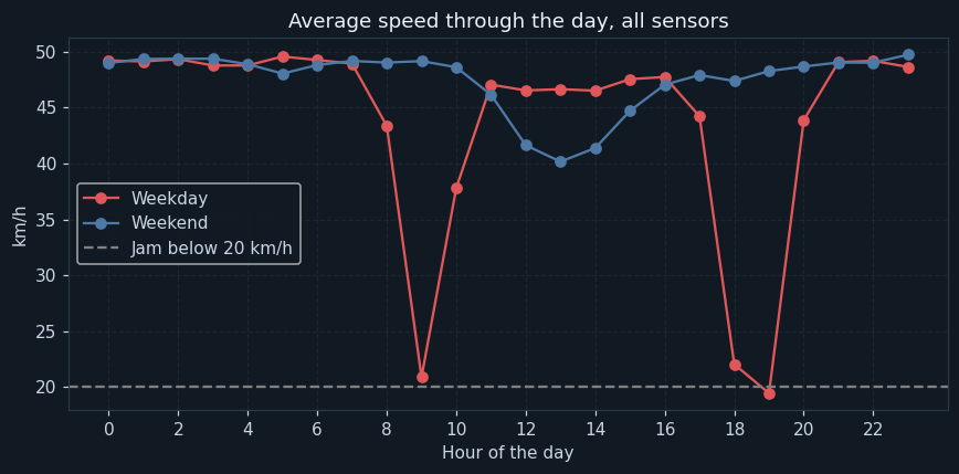
The average speed at every hour, over all sensors, for weekdays and weekends — computed by map-and-reduce from the chunks.
Weekdays have two dips: the morning and the evening rush. The evening is deeper, falling near the 20 km/h jam line on average. Weekends only slow gently around midday.
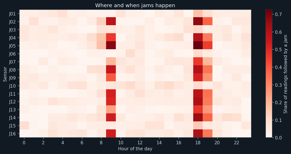
Each cell is one sensor at one hour; the darker the red, the more of its readings were followed by a jam.
Jams are concentrated at the two rush hours on most sensors, worst at J05. A few roads, such as J01, J06, J10 and J15, rarely jam at all. The faint red at other hours is accidents.
7Step 6 — Data Preparation
Removed by time and sensor in each chunk — including against the previous chunk's last readings, so a duplicate that straddles a chunk edge is caught too.
Treated as missing, then filled with that sensor's previous reading. Five minutes earlier is the best estimate of a road's speed.
Filled with that sensor's previous count, in the same way.
The last three readings of every sensor are carried into the next chunk, so the 15-minute change can be worked out at the edges too. Only each sensor's very first three readings are lost.
Feature engineering
speed_drop_15min is how much the speed has fallen in the last fifteen minutes. A road slowing down fast is about to jam; a road that is slow but steady may not be. It needs the carry between chunks.
rush_hour marks weekday readings from 8 to 11 am and 5 to 9 pm; weekend marks Saturdays and Sundays. They let the models learn the daily pattern without being given the exact clock time.
After cleaning, 128928 readings remain. The first three weeks — 96720 readings, of which 6925 were followed by a jam — are used for training; the last week, 32208 readings, for testing, as it would be used: on days it has not seen.
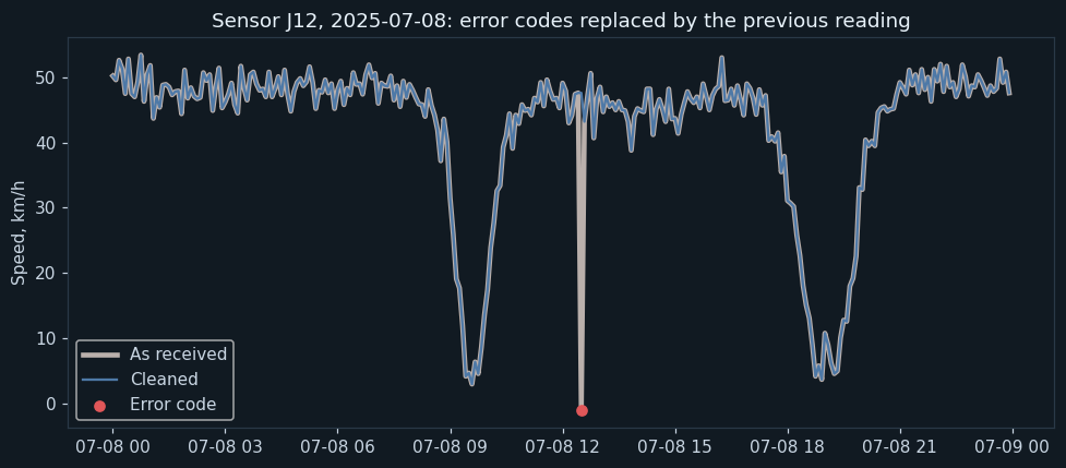
One day at the sensor with the most error codes in the first chunk. The thick grey line is the speeds as received, the blue line after cleaning, and the red dot an error code.
Left in, the -1 would look like a road suddenly at a standstill — and a 255 elsewhere in the data like a car flying past at 255 km/h. Either would teach the model nonsense. Replacing each with the sensor's previous reading leaves a believable line, and the rest of the day is untouched.
8Step 7 — Modelling
Each historical reading has a known outcome — jammed fifteen minutes later or not — so this is supervised binary classification.
The split is by time, not random: the first three weeks to train and the last week to test. A random split would let the model learn from minutes on both sides of a test reading, which never happens in real use.
How the models work
The online model is logistic regression trained by SGDClassifier. Its partial_fit method takes one chunk at a time and nudges the model's weights; three passes are made over the stream. A StandardScaler is fitted bit by bit in the same way. Because jams are rare, a jam reading is given a weight of 13.0 (for the online model), worked out from the class counts gathered while streaming.
The second approach takes a random 10% of each training chunk — a sample small enough to hold in memory — and trains a Random Forest of 200 trees on it, with balanced class weights.
The rule needs no training: it warns if the road is already jammed.
9Step 8 — Evaluation
On the test week, precision, recall and F1 were: rule 0.701 , 0.701 , 0.701; online model 0.412 , 0.884 , 0.562; Random Forest 0.649 , 0.828 , 0.728.
Those scores hide what the control room cares about. A jam that has already started needs no warning — the operator can see it. What matters is the readings where the road was still clear but jammed fifteen minutes later: 704 of them. The rule warned of 0 (0%) — by its nature it can only report jams that exist. The online model warned of 430 (61%), but with 2266 false alarms on clear roads; the forest warned of 318 (45%) with 420 false alarms.
The forest, trained on just a tenth of the data, has the best F1 and, on roads that were still clear, about a fifth of the online model's false alarms. More data did not beat a better-suited model: the link between speed, occupancy and jams is not a straight line, and logistic regression can only draw straight lines. The operator was clear that too many false alarms make warnings useless, so the forest is deployed.
Chart 5 shows the limit. In rush hours the forest warned of 0.618 of new jams; at other times only 0.145. Those are mostly accidents, which nothing in the sensor data can foresee.
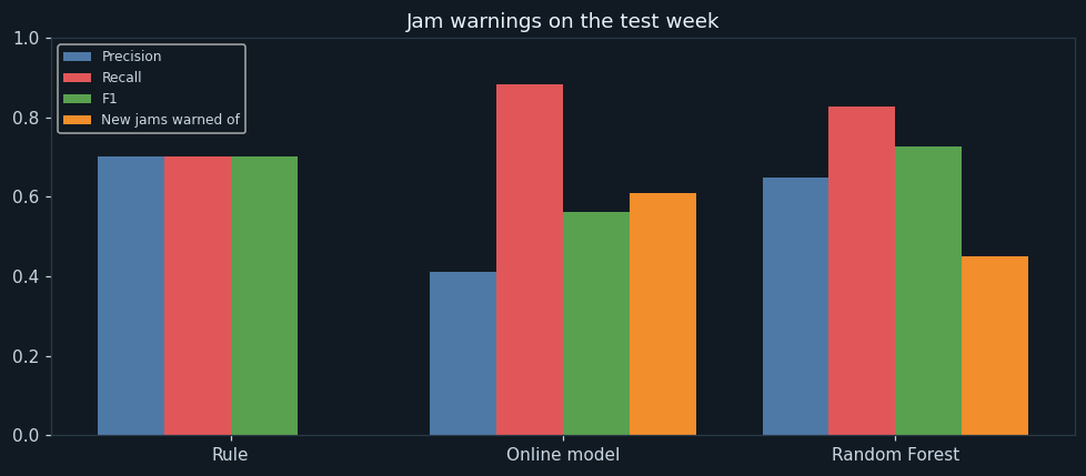
For each approach on the test week: precision, recall, F1, and the share of new jams warned of before they started.
The rule's F1 looks respectable, but its orange bar is empty: it never warns before a jam starts. The online model warns of the most new jams but has the lowest precision. The forest has the best F1 and still warns of almost half the new jams.
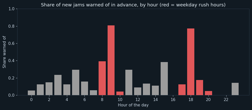
For the forest, the share of new jams warned of at each hour; red bars are weekday rush hours.
Rush-hour jams build up gradually, so the forest warns of most of them. Jams at other hours are mostly sudden accidents, with nothing in the data to give them away — the constable's point exactly.
10Step 9 — Deployment
The forest is saved to jam_model.pkl. In use, each new reading is cleaned as it arrives — using the carried readings for the 15-minute change — and given to the model; a 'jam likely' answer flashes a warning for that junction on the control-room screen.
The program replays an evening at sensor J05 one reading at a time: 85 readings streamed. The first warning came at 2025-07-30 17:55; the road first jammed at 2025-07-30 18:15. 21 warnings were issued in all, most of them while the jam lasted.
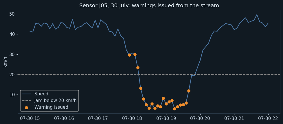
Sensor J05's speed from 3 to 10 pm on a test evening, with an orange dot for each warning issued as the readings arrived.
The first warning comes while the road is still moving at about 30 km/h, before it falls below the jam line. Warnings continue while the jam lasts and stop as it clears.
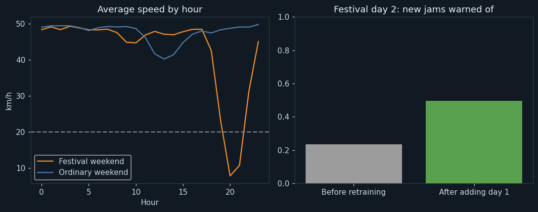
Left: average speed by hour on the festival days and on an ordinary weekend. Right: the share of new jams on festival day 2 warned of, before and after retraining with day 1.
Festival shopping brings a deep jam in the evening, on a weekend, when the model expects quiet roads. Adding day 1 to the training sample doubles the share of day 2's new jams warned of.
11Step 10 — Feedback
Patterns change — the variability of big data. Festival-shopping days were the test: heavy evening crowds on a weekend, when the training data says roads are quiet. On festival day 1 the deployed forest warned of only 0.188 of new jams.
Labels for day 1 are known by the next morning, so day 1 was added to the training sample and the forest retrained. On festival day 2, the share of new jams warned of rose from 0.234 to 0.495, and recall from 0.859 to 0.907.
The lesson for running the system: retrain regularly on a fresh sample that includes recent days, and before known festivals, add last year's festival days. An online model could do the same by calling partial_fit on each day's labelled data — learning continuously without storing the data at all.
12Ethical considerations
Road sensors count vehicles and measure speed; they do not identify anyone. If cameras or phone data were added, number plates and locations of people would need strict protection.
Areas with more sensors get better warnings. Poorer neighbourhoods with fewer sensors should not be left with worse traffic management.
The model cannot foresee accidents. Operators must keep watching the screens and not treat 'no warning' as 'no problem'.
Signal changes made because of a warning should never delay an ambulance or fire engine.
13Source code
The whole program, laid out as the ten steps of the methodology. Every chart and number on this page came out of running it.
# ---------------------------------------------------------------------------
# traffic_stream.py
#
# Capstone project: warning a city's traffic control room fifteen minutes
# before a road jams, from a non-stop stream of sensor readings.
#
# CBSE Class XII, Artificial Intelligence (843), Part C - Capstone Project.
# SDG 11 (Sustainable Cities and Communities).
#
# Data Science Methodology, 10 steps, with BIG DATA ideas: the file is never
# loaded whole. It is read in chunks, summarised map-and-reduce style, cleaned
# chunk by chunk, and learned from in two big-data ways: an online model
# (partial_fit) that learns from every chunk in turn, and a Random Forest
# trained on a 10% sample. Both are compared with a simple rule.
#
# Libraries: pandas, numpy, matplotlib, scikit-learn, joblib.
# ---------------------------------------------------------------------------

# %% Step 1 - Business Understanding
print("=" * 64)
print("TRAFFIC JAM EARLY WARNING")
print("=" * 64)
print("Problem : by the time the control room sees a jam, it has already formed")
print("Goal    : warn 15 minutes ahead, so signals can be retimed and traffic")
print("          diverted while it still helps")
print()

# %% Step 2 - Analytic Approach
print("Analytic approach : predictive - will this road jam in 15 minutes? (yes/no)")
print("Jam means         : average speed below 20 km/h")
print()

# %% Step 3 - Data Requirements
import os
import pandas as pd
import numpy as np
import matplotlib.pyplot as plt
from sklearn.preprocessing import StandardScaler
from sklearn.linear_model import SGDClassifier
from sklearn.ensemble import RandomForestClassifier
import joblib

FILE = "traffic_sensors.csv"
CHUNK = 20000                      # rows held in memory at a time
TEST_FROM = "2025-07-28"           # the last week is kept for testing
FEATURES = ["speed_kmph", "speed_drop_15min", "vehicles", "occupancy_pct", "rush_hour", "weekend"]

# %% Step 4 - Data Collection
print("--- Step 4: Data Collection ---")
print("File size :", round(os.path.getsize(FILE) / 1e6, 1), "MB")
rows = 0
chunks = 0
for chunk in pd.read_csv(FILE, chunksize=CHUNK):
    rows = rows + len(chunk)
    chunks = chunks + 1
print("Readings  :", rows)
print("Read in", chunks, "chunks of at most", CHUNK, "rows - never all at once")
print()

# %% Step 5 - Data Understanding
# MAP: summarise each chunk on its own. REDUCE: add the summaries together.
print("--- Step 5: Data Understanding ---")
speed_total = None
error_codes = 0
blank_counts = 0
jam_total = None
for chunk in pd.read_csv(FILE, chunksize=CHUNK):
    bad = (chunk["speed_kmph"] < 0) | (chunk["speed_kmph"] > 150)
    error_codes = error_codes + int(bad.sum())
    blank_counts = blank_counts + int(chunk["vehicles"].isnull().sum())
    good = chunk[~bad].copy()
    t = pd.to_datetime(good["time"])
    good["hour"] = t.dt.hour
    good["day"] = np.where(t.dt.dayofweek >= 5, "Weekend", "Weekday")
    part = good.groupby(["day", "hour"])["speed_kmph"].agg(["sum", "count"])           # map
    speed_total = part if speed_total is None else speed_total.add(part, fill_value=0)  # reduce
    jams = good.groupby(["sensor", "hour"])["jam_in_15_min"].agg(["sum", "count"])
    jam_total = jams if jam_total is None else jam_total.add(jams, fill_value=0)
avg_speed = (speed_total["sum"] / speed_total["count"]).unstack(0)
jam_share = (jam_total["sum"] / jam_total["count"]).unstack(1)
overall = jam_total["sum"].sum() / jam_total["count"].sum()
print("Speed error codes (-1 or 255) :", error_codes)
print("Blank vehicle counts          :", blank_counts)
print("Readings followed by a jam    :", round(100 * overall, 1), "%")
print("Slowest weekday hour          :", str(int(avg_speed["Weekday"].idxmin())) + ":00, average",
      round(avg_speed["Weekday"].min(), 1), "km/h")
print("Slowest weekend hour          :", str(int(avg_speed["Weekend"].idxmin())) + ":00, average",
      round(avg_speed["Weekend"].min(), 1), "km/h")
print("Sensor with the most jams     :", jam_share.mean(axis=1).idxmax())
print()

# Chart 1: average speed through the day.
plt.figure(figsize=(8, 4))
plt.plot(avg_speed.index, avg_speed["Weekday"], marker="o", label="Weekday", color="#e15759")
plt.plot(avg_speed.index, avg_speed["Weekend"], marker="o", label="Weekend", color="#4e79a7")
plt.axhline(20, color="gray", linestyle="--", label="Jam below 20 km/h")
plt.title("Average speed through the day, all sensors")
plt.xlabel("Hour of the day")
plt.ylabel("km/h")
plt.xticks(range(0, 24, 2))
plt.legend()
plt.grid(True, linestyle="--", alpha=0.4)
plt.tight_layout()
plt.savefig("chart1_hourly_speed.png")
plt.close()

# Chart 2: where and when jams follow.
plt.figure(figsize=(10, 5))
plt.imshow(jam_share.values, cmap="Reds", aspect="auto")
plt.colorbar(label="Share of readings followed by a jam")
plt.yticks(range(len(jam_share)), jam_share.index)
plt.xticks(range(0, 24, 2))
plt.xlabel("Hour of the day")
plt.ylabel("Sensor")
plt.title("Where and when jams happen")
plt.tight_layout()
plt.savefig("chart2_jam_heatmap.png")
plt.close()

# %% Step 6 - Data Preparation
# Each chunk is cleaned on its own. A chunk's first rows need the readings
# just before them (for the 15-minute change), so the last three readings of
# every sensor are CARRIED from one chunk to the next.
print("--- Step 6: Data Preparation ---")


def prepare(chunk, carry):
    chunk = chunk.copy()
    chunk["new"] = True
    both = pd.concat([carry, chunk])
    before = len(both)
    both = both.drop_duplicates(subset=["time", "sensor"])
    duplicates = before - len(both)
    bad = (both["speed_kmph"] < 0) | (both["speed_kmph"] > 150)
    both.loc[bad, "speed_kmph"] = np.nan
    both = both.sort_values(["sensor", "time"], kind="stable")
    # An error code or a blank count is replaced by that sensor's previous reading.
    both["speed_kmph"] = both.groupby("sensor")["speed_kmph"].ffill()
    both["vehicles"] = both.groupby("sensor")["vehicles"].ffill()
    both["speed_drop_15min"] = both.groupby("sensor")["speed_kmph"].shift(3) - both["speed_kmph"]
    t = pd.to_datetime(both["time"])
    both["weekend"] = (t.dt.dayofweek >= 5).astype(int)
    both["rush_hour"] = (t.dt.hour.isin([8, 9, 10, 17, 18, 19, 20]) & (both["weekend"] == 0)).astype(int)
    new_carry = both.groupby("sensor").tail(3).drop(columns="speed_drop_15min").assign(new=False)
    ready = both[both["new"] & both["speed_drop_15min"].notna()].sort_values(["time", "sensor"])
    return ready, new_carry, duplicates


def stream(file):
    """Yield one cleaned chunk at a time."""
    carry = pd.DataFrame()
    for chunk in pd.read_csv(file, chunksize=CHUNK):
        ready, carry, duplicates = prepare(chunk, carry)
        yield ready, duplicates


scaler = StandardScaler()
counts = np.zeros(2)
sample = []
duplicates_removed = 0
cleaned_rows = 0
for ready, dups in stream(FILE):
    duplicates_removed = duplicates_removed + dups
    cleaned_rows = cleaned_rows + len(ready)
    train = ready[ready["time"] < TEST_FROM]
    if len(train) > 0:
        scaler.partial_fit(train[FEATURES])                       # learns means bit by bit
        counts = counts + np.bincount(train["jam_in_15_min"], minlength=2)
        sample.append(train.sample(frac=0.1, random_state=0))    # a 10% sample for the forest
print("Readings sent twice, removed   :", duplicates_removed)
print("Error codes and blanks         : replaced by the sensor's previous reading")
print("Clean readings                 :", cleaned_rows)
print("Training readings (3 weeks)    :", int(counts.sum()))
print("  of which followed by a jam   :", int(counts[1]))
weight = counts[0] / counts[1]
print("Weight given to a jam reading  :", round(weight, 1), "(for the online model)")
print()

# Chart 3: one day at the sensor with the most error codes, before and after cleaning.
raw = pd.read_csv(FILE, nrows=CHUNK)
clean0, _, _ = prepare(raw, pd.DataFrame())
faulty = raw[(raw["speed_kmph"] < 0) | (raw["speed_kmph"] > 150)]
bad_sensor = faulty["sensor"].value_counts().index[0] if len(faulty) > 0 else raw["sensor"].iloc[0]
day = faulty[faulty["sensor"] == bad_sensor]["time"].iloc[0][:10] if len(faulty) > 0 else raw["time"].iloc[0][:10]
r = raw[(raw["sensor"] == bad_sensor) & raw["time"].str.startswith(day)].drop_duplicates(subset="time")
c = clean0[(clean0["sensor"] == bad_sensor) & clean0["time"].str.startswith(day)]
e = r[(r["speed_kmph"] < 0) | (r["speed_kmph"] > 150)]
plt.figure(figsize=(9, 4))
plt.plot(pd.to_datetime(r["time"]), r["speed_kmph"], color="#bab0ac", linewidth=3, label="As received")
plt.plot(pd.to_datetime(c["time"]), c["speed_kmph"], color="#4e79a7", label="Cleaned")
plt.scatter(pd.to_datetime(e["time"]), e["speed_kmph"], color="#e15759", zorder=3, label="Error code")
plt.title("Sensor " + bad_sensor + ", " + day + ": error codes replaced by the previous reading")
plt.ylabel("Speed, km/h")
plt.legend()
plt.tight_layout()
plt.savefig("chart3_cleaning.png")
plt.close()

# %% Step 7 - Modelling
print("--- Step 7: Modelling ---")
# average=True keeps a running average of the weights, so the online model
# does not swing with whichever chunk it saw last.
online = SGDClassifier(loss="log_loss", class_weight={0: 1, 1: weight}, average=True, random_state=0)
for epoch in range(3):                                            # three passes over the stream
    for ready, _ in stream(FILE):
        train = ready[ready["time"] < TEST_FROM]
        if len(train) > 0:
            online.partial_fit(scaler.transform(train[FEATURES]), train["jam_in_15_min"], classes=[0, 1])
print("Online model    : logistic regression learned with partial_fit, chunk by chunk, 3 passes")
small = pd.concat(sample)
forest = RandomForestClassifier(n_estimators=200, min_samples_leaf=5, class_weight="balanced", random_state=0)
forest.fit(small[FEATURES], small["jam_in_15_min"])
print("Random Forest   : trained on a 10% sample of", len(small), "readings held in memory")
print("Rule            : warn if the road is already jammed now")
print("Online model weights:")
for f, w in zip(FEATURES, online.coef_[0]):
    print("  ", f.ljust(18), round(w, 2))
print()

# %% Step 8 - Evaluation
print("--- Step 8: Evaluation ---")
names = ["Rule", "Online model", "Random Forest"]
tally = {n: np.zeros((2, 2), dtype=int) for n in names}          # [true][predicted]
onset = {n: np.zeros(3, dtype=int) for n in names}               # new jams warned, new jams, false alarms
by_hour = np.zeros((24, 2))                                       # jams caught, jams total
test_rows = 0
for ready, _ in stream(FILE):
    test = ready[ready["time"] >= TEST_FROM]
    if len(test) == 0:
        continue
    test_rows = test_rows + len(test)
    y = test["jam_in_15_min"].values
    clear = (test["speed_kmph"] >= 20).values                     # not jammed yet
    preds = {"Rule": (test["speed_kmph"] < 20).astype(int).values,
             "Online model": online.predict(scaler.transform(test[FEATURES])),
             "Random Forest": forest.predict(test[FEATURES])}
    for n in names:
        for a in (0, 1):
            for b in (0, 1):
                tally[n][a, b] += int(((y == a) & (preds[n] == b)).sum())
        onset[n] += [int((clear & (y == 1) & (preds[n] == 1)).sum()), int((clear & (y == 1)).sum()),
                     int((clear & (y == 0) & (preds[n] == 1)).sum())]
    hours = pd.to_datetime(test["time"]).dt.hour.values
    for h in range(24):
        jam = (hours == h) & (y == 1) & clear
        by_hour[h, 0] += (preds["Random Forest"][jam] == 1).sum()
        by_hour[h, 1] += jam.sum()
print("Test readings (last week) :", test_rows)
scores = {}
for n in names:
    tn, fp, fn, tp = tally[n].ravel()
    p = tp / (tp + fp)
    r = tp / (tp + fn)
    scores[n] = [p, r, 2 * p * r / (p + r), onset[n][0] / onset[n][1]]
    print(n.ljust(14), " TP", tp, " FN", fn, " FP", fp, " TN", tn)
print()
print("Model           precision  recall    F1")
for n in names:
    print(f"{n:<15} {scores[n][0]:9.3f} {scores[n][1]:7.3f} {scores[n][2]:6.3f}")
for n in names:
    print("Precision, recall, F1 -", n, ":", round(scores[n][0], 3), ",", round(scores[n][1], 3), ",", round(scores[n][2], 3))
print()
print("A warning matters most BEFORE a jam starts. Readings where the road")
print("was still clear but jammed 15 minutes later:", onset["Rule"][1])
for n in names:
    print(n + ", new jams warned of :", onset[n][0], "(" + str(round(100 * scores[n][3])) + "%)")
    print(n + ", false alarms on clear roads :", onset[n][2])
best = max(["Online model", "Random Forest"], key=lambda n: scores[n][2])
print("Best F1 :", best)
print()
rush = [8, 9, 10, 17, 18, 19, 20]
calm = [h for h in range(24) if h not in rush]
for label, hrs in [("in rush hours ", rush), ("at other times", calm)]:
    if by_hour[hrs, 1].sum() > 0:
        print("Random Forest, new jams warned of", label, ":", round(by_hour[hrs, 0].sum() / by_hour[hrs, 1].sum(), 3))
    else:
        print("Random Forest, new jams warned of", label, ": no new jams at these times")
print()

# Chart 4: the three approaches compared.
x = np.arange(3)
plt.figure(figsize=(9, 4))
labels = [("Precision", "#4e79a7"), ("Recall", "#e15759"), ("F1", "#59a14f"), ("New jams warned of", "#f28e2b")]
for k, (label, colour) in enumerate(labels):
    plt.bar(x + (k - 1.5) * 0.2, [scores[n][k] for n in names], width=0.2, label=label, color=colour)
plt.xticks(x, names)
plt.ylim(0, 1)
plt.title("Jam warnings on the test week")
plt.legend(loc="upper left", fontsize=8)
plt.tight_layout()
plt.savefig("chart4_models.png")
plt.close()

# Chart 5: which new jams the forest warns of, by hour.
plt.figure(figsize=(9, 4))
share = by_hour[:, 0] / np.maximum(by_hour[:, 1], 1)
plt.bar(range(24), share, color=["#e15759" if h in rush else "#9c9c9c" for h in range(24)])
plt.title("Share of new jams warned of in advance, by hour (red = weekday rush hours)")
plt.xlabel("Hour of the day")
plt.ylabel("Share warned of")
plt.xticks(range(0, 24, 2))
plt.ylim(0, 1)
plt.tight_layout()
plt.savefig("chart5_recall_by_hour.png")
plt.close()

# %% Step 9 - Deployment
# The saved model reads the stream as it arrives, and warns on the fly.
print("--- Step 9: Deployment ---")
joblib.dump(forest, "jam_model.pkl")
model = joblib.load("jam_model.pkl")
evening = None
for ready, _ in stream(FILE):
    part = ready[(ready["sensor"] == "J05") & (ready["time"] >= "2025-07-30 15:00") & (ready["time"] <= "2025-07-30 22:00")]
    if len(part) > 0:
        evening = part if evening is None else pd.concat([evening, part])
alerts = []
for i in range(len(evening)):
    reading = evening.iloc[[i]]                                   # one reading arrives
    if model.predict(reading[FEATURES])[0] == 1:
        alerts.append(reading["time"].iloc[0])
print("Sensor J05, 30 July, 3 pm to 10 pm :", len(evening), "readings streamed")
print("Warnings issued                    :", len(alerts))
print("First warning                      :", alerts[0] if alerts else "none")
jam_times = evening[evening["speed_kmph"] < 20]["time"]
print("Road first jammed                  :", jam_times.iloc[0] if len(jam_times) else "never")
print()

# Chart 6: the evening, as the control room would have seen it.
t = pd.to_datetime(evening["time"])
plt.figure(figsize=(9, 4))
plt.plot(t, evening["speed_kmph"], color="#4e79a7", label="Speed")
plt.axhline(20, color="gray", linestyle="--", label="Jam below 20 km/h")
warned = evening["time"].isin(alerts)
plt.scatter(t[warned], evening["speed_kmph"][warned], color="#f28e2b", zorder=3, label="Warning issued")
plt.title("Sensor J05, 30 July: warnings issued from the stream")
plt.ylabel("km/h")
plt.legend()
plt.tight_layout()
plt.savefig("chart6_stream_evening.png")
plt.close()

# %% Step 10 - Feedback
# Two festival shopping days, on a weekend: crowds when the model expects a
# quiet road. Day 1 is added to the training sample, and day 2 checked again.
print("--- Step 10: Feedback ---")
fest, _ = next(stream("festival_days.csv"))
day1 = fest[fest["time"] < "2025-10-19"]
day2 = fest[fest["time"] >= "2025-10-19"]


def check(m, d):
    p = m.predict(d[FEATURES])
    y = d["jam_in_15_min"].values
    clear = (d["speed_kmph"] >= 20).values
    return ((p == 1) & (y == 1)).sum() / (y == 1).sum(), ((p == 1) & (y == 1) & clear).sum() / ((y == 1) & clear).sum()


print("Festival day 1, new jams warned of :", round(check(model, day1)[1], 3))
r_before, n_before = check(model, day2)
print("Festival day 2 before retraining, recall             :", round(r_before, 3))
print("Festival day 2 before retraining, new jams warned of :", round(n_before, 3))
small2 = pd.concat([small, day1])
model2 = RandomForestClassifier(n_estimators=200, min_samples_leaf=5, class_weight="balanced", random_state=0)
model2.fit(small2[FEATURES], small2["jam_in_15_min"])
r_after, n_after = check(model2, day2)
print("Festival day 2 after adding day 1, recall             :", round(r_after, 3))
print("Festival day 2 after adding day 1, new jams warned of :", round(n_after, 3))

# Chart 7: festival days against an ordinary weekend, and the retraining.
plt.figure(figsize=(10, 4))
plt.subplot(1, 2, 1)
fh = pd.to_datetime(fest["time"]).dt.hour
plt.plot(fest.groupby(fh)["speed_kmph"].mean(), color="#f28e2b", label="Festival weekend")
plt.plot(avg_speed["Weekend"], color="#4e79a7", label="Ordinary weekend")
plt.axhline(20, color="gray", linestyle="--")
plt.title("Average speed by hour")
plt.xlabel("Hour")
plt.ylabel("km/h")
plt.legend()
plt.subplot(1, 2, 2)
plt.bar(["Before retraining", "After adding day 1"], [n_before, n_after], color=["#9c9c9c", "#59a14f"])
plt.ylim(0, 1)
plt.title("Festival day 2: new jams warned of")
plt.tight_layout()
plt.savefig("chart7_festival.png")
plt.close()
The library calls it is built from
| Call | Step | What it does |
|---|---|---|
pd.read_csv(chunksize=20000) | Steps 4–10 | Reads the file one chunk at a time |
groupby().agg(["sum", "count"]) then add() | Step 5 | Map-and-reduce summaries across chunks |
drop_duplicates(subset=["time", "sensor"]) | Step 6 | Removes readings sent twice |
groupby("sensor").ffill() | Step 6 | Fills error codes and blanks from the previous reading |
groupby("sensor").tail(3) | Step 6 | The carry between chunks |
StandardScaler().partial_fit() | Step 6 | Learns the scaling bit by bit |
SGDClassifier(loss="log_loss").partial_fit() | Step 7 | Online logistic regression, one chunk at a time |
DataFrame.sample(frac=0.1) | Step 6 | The 10% sample for the forest |
RandomForestClassifier(class_weight="balanced") | Step 7 | The forest |
joblib.dump() / load() | Step 9 | Saves and reloads the model |
14Output of a real run
================================================================
TRAFFIC JAM EARLY WARNING
================================================================
Problem : by the time the control room sees a jam, it has already formed
Goal    : warn 15 minutes ahead, so signals can be retimed and traffic
          diverted while it still helps

Analytic approach : predictive - will this road jam in 15 minutes? (yes/no)
Jam means         : average speed below 20 km/h

--- Step 4: Data Collection ---
File size : 4.6 MB
Readings  : 129066
Read in 7 chunks of at most 20000 rows - never all at once

--- Step 5: Data Understanding ---
Speed error codes (-1 or 255) : 140
Blank vehicle counts          : 60
Readings followed by a jam    : 7.2 %
Slowest weekday hour          : 19:00, average 19.4 km/h
Slowest weekend hour          : 13:00, average 40.2 km/h
Sensor with the most jams     : J05

--- Step 6: Data Preparation ---
Readings sent twice, removed   : 90
Error codes and blanks         : replaced by the sensor's previous reading
Clean readings                 : 128928
Training readings (3 weeks)    : 96720
  of which followed by a jam   : 6925
Weight given to a jam reading  : 13.0 (for the online model)

--- Step 7: Modelling ---
Online model    : logistic regression learned with partial_fit, chunk by chunk, 3 passes
Random Forest   : trained on a 10% sample of 9672 readings held in memory
Rule            : warn if the road is already jammed now
Online model weights:
   speed_kmph         -3.64
   speed_drop_15min   2.79
   vehicles           -0.07
   occupancy_pct      4.75
   rush_hour          -0.17
   weekend            -0.53

--- Step 8: Evaluation ---
Test readings (last week) : 32208
Rule            TP 1649  FN 704  FP 703  TN 29152
Online model    TP 2079  FN 274  FP 2969  TN 26886
Random Forest   TP 1949  FN 404  FP 1053  TN 28802

Model           precision  recall    F1
Rule                0.701   0.701  0.701
Online model        0.412   0.884  0.562
Random Forest       0.649   0.828  0.728
Precision, recall, F1 - Rule : 0.701 , 0.701 , 0.701
Precision, recall, F1 - Online model : 0.412 , 0.884 , 0.562
Precision, recall, F1 - Random Forest : 0.649 , 0.828 , 0.728

A warning matters most BEFORE a jam starts. Readings where the road
was still clear but jammed 15 minutes later: 704
Rule, new jams warned of : 0 (0%)
Rule, false alarms on clear roads : 0
Online model, new jams warned of : 430 (61%)
Online model, false alarms on clear roads : 2266
Random Forest, new jams warned of : 318 (45%)
Random Forest, false alarms on clear roads : 420
Best F1 : Random Forest

Random Forest, new jams warned of in rush hours  : 0.618
Random Forest, new jams warned of at other times : 0.145

--- Step 9: Deployment ---
Sensor J05, 30 July, 3 pm to 10 pm : 85 readings streamed
Warnings issued                    : 21
First warning                      : 2025-07-30 17:55
Road first jammed                  : 2025-07-30 18:15

--- Step 10: Feedback ---
Festival day 1, new jams warned of : 0.188
Festival day 2 before retraining, recall             : 0.859
Festival day 2 before retraining, new jams warned of : 0.234
Festival day 2 after adding day 1, recall             : 0.907
Festival day 2 after adding day 1, new jams warned of : 0.49515The same project in Orange
Orange cannot stream a file in chunks, so the no-code version works on a sample — which is itself one of the big data techniques in this project. The tool is Orange Data Mining.
| Widget | What it does |
|---|---|
| File | Load traffic_sensors.csv (a sample of it, for very large files). |
| Data Sampler | Take a 10% random sample — the same idea as the forest in the program. |
| Feature Constructor | Add rush_hour and weekend; set jam_in_15_min as the target. |
| Logistic Regression and Random Forest | Connect both to Test and Score. |
| Test and Score | Compare precision, recall and F1 for class 1. |
| Confusion Matrix | Count jams missed and false alarms. |
16Testing
Every case was run: each gives the whole program a small input of its own.
| Test case | Expected | Actual | Result |
|---|---|---|---|
| The whole file is counted, chunk by chunk | Readings : 129066 | Readings : 129066 | Pass |
| Speed error codes are found by the streamed summary | Speed error codes (-1 or 255) : 140 | Speed error codes (-1 or 255) : 140 | Pass |
| Readings sent twice are removed | Readings sent twice, removed : 90 | Readings sent twice, removed : 90 | Pass |
| The rule cannot warn of a jam before it starts | Rule, new jams warned of : 0 (0%) | Rule, new jams warned of : 0 (0%) | Pass |
| The forest from a 10% sample has the best F1 | Best F1 : Random Forest | Best F1 : Random Forest | Pass |
| Learning from festival day 1 helps on day 2 | Festival day 2 after adding day 1, new jams warned of : 0.495 | Festival day 2 after adding day 1, new jams warned of : 0.495 | Pass |
| No readings are lost at chunk edges (only each sensor's first three) | Clean readings : 20154 | Clean readings : 20154 | Pass |
| A jam every weekday at 6 pm: every new jam warned of - but rush hour alone also raises false alarms | Random Forest, new jams warned of : 12 (100%) / Random Forest, false alarms on clear roads : 600 | Random Forest, new jams warned of : 12 (100%) / Random Forest, false alarms on clear roads : 600 | Pass |
| Five error codes are counted | Speed error codes (-1 or 255) : 5 | Speed error codes (-1 or 255) : 5 | Pass |
| The data file is missing | FileNotFoundError: [Errno 2] No such file or directory: 'traffic_sensors.csv' | FileNotFoundError: [Errno 2] No such file or directory: 'traffic_sensors.csv' | Pass |
17Team roles and timeline
A capstone is done by a group of 3 to 5. A suggested split of the work, and a timeline across the year:
| Role | Responsible for |
|---|---|
| Project lead | Business understanding; interviews at the control room and with a constable |
| Data engineer | Chunked reading, the carry between chunks, and veracity checks |
| Analyst | Map-and-reduce summaries, the heat map and the big data characteristics |
| Modeller | The online model, the sampled forest and the evaluation of new jams |
| Documentation and video | The report, the stream replay, the festival test and the video |
| When | Methodology steps | Deliverable |
|---|---|---|
| June | 1 Business Understanding, 2 Analytic Approach | Problem statement; control-room visit |
| July | 3 Data Requirements, 4 Data Collection | Four weeks of sensor data |
| August | 5 Data Understanding, 6 Data Preparation | Chunked summaries; cleaning with the carry |
| September | 7 Modelling, 8 Evaluation | Three approaches compared on new jams |
| October – November | 9 Deployment, 10 Feedback | Stream replay; festival days tested |
| December – January | Documentation and video | Report and 3-minute video |
18Results, limits and what next
- 129066 readings were handled in chunks without ever loading the file whole.
- The rule warned of 0 (0%) new jams — it can only see jams that have started.
- A Random Forest on a 10% sample beat an online model trained on everything: F1 0.649 , 0.828 , 0.728 (precision, recall, F1).
- Rush-hour jams are warned of far more often than accident jams.
- Retraining with festival day 1 raised the share of day 2's new jams warned of from 0.234 to 0.495.
Limitations
- Sample data for sixteen imaginary sensors
- Accidents cannot be foreseen from speed data
- Each sensor is predicted on its own; jams spread from road to road
- Fifteen minutes ahead only
Future scope
- Use neighbouring sensors' readings, since jams spread upstream
- Add rain, events and holidays as features
- Use a big data platform such as Apache Spark for a whole city's stream
- Connect warnings directly to adaptive signal timing
What the team had to learn
- The characteristics of big data: volume, velocity, variety, veracity, variability and value
- Reading data in chunks with pandas
- Map-and-reduce style summaries
- Online learning with partial_fit, and sampling
- Why the right measure matters: warning before the event, not after
19Conclusion
The capstone built a jam warning from a stream of sensor data without ever holding the data all at once: chunks, map-and-reduce summaries, cleaning with a carry between chunks, and two ways of learning from data too large for memory.
Its most useful lesson came from choosing the right measure. A rule that only reports existing jams scored a respectable F1 and warned of none of them in advance. Counting warnings before a jam starts showed what each approach was really worth.
A forest trained on a tenth of the data won, because it fitted the problem better — more data is not always the answer. And the festival test showed that a model is never finished: patterns change, and retraining on recent days keeps it useful.
20The 3-minute video script
Part C asks for a video of exactly three minutes with six parts. A script, timed to the second:
| Time | Part | What to say and show |
|---|---|---|
| 0:00 – 0:25 | a. Problem statement | Show a jammed junction. "By the time the control room sees a jam, it has already formed." |
| 0:25 – 0:40 | b. SDG alignment | SDG 11 icon. "Sustainable transport, cleaner air and faster emergency trips." |
| 0:40 – 1:15 | c. AI concepts and algorithms | "Big data: a stream read in chunks, map-and-reduce summaries, and two ways to learn from it — an online model with partial_fit and a Random Forest on a sample." |
| 1:15 – 2:15 | d. How it works | Show the chunk counter, then chart 4: the rule warns of no jams before they start. Then chart 6: warnings arriving before J05 jams. |
| 2:15 – 2:45 | e. Conclusion | "Most rush-hour jams warned of in advance; accidents still cannot be foreseen." |
| 2:45 – 3:00 | f. Acknowledgement | "We thank our AI teacher, [name], and the traffic control room staff." |
21Questions for the viva
▸Why read the file in chunks?
Big data can be too large to fit in memory. Reading chunks of 20,000 rows means the same program works on a file of any size.
▸What does map-and-reduce mean in your program?
Each chunk is summarised on its own (map) — total speed and count per hour — and the summaries are added together (reduce).
▸Why carry readings between chunks?
The 15-minute speed change needs earlier readings. Without the carry, the first rows of every chunk would have no change and be lost.
▸What does partial_fit do?
It updates the model with one chunk of data, so the model can learn from data that never fits in memory — and keep learning as new data arrives.
▸Why did the rule warn of no new jams?
It warns only when the road is already jammed, so it can never warn before a jam starts.
▸Why did a forest on 10% of the data beat the online model on all of it?
Jams depend on speed and occupancy in a curved way, which logistic regression cannot capture. The better-suited model mattered more than the amount of data.
▸Which characteristics of big data does your data show?
Volume, velocity, variety, veracity (error codes and duplicates), variability (festivals) and value (the warning).
▸Which SDG does it align to?
SDG 11, Sustainable Cities and Communities — target 11.2 on transport and 11.6 on air quality.
22References
- Smart Cities Mission, Ministry of Housing and Urban Affairs — https://smartcities.gov.in/
- pandas: iterating through files chunk by chunk — https://pandas.pydata.org/docs/user_guide/io.html#io-chunking
- scikit-learn: SGDClassifier and incremental learning — https://scikit-learn.org/stable/computing/scaling_strategies.html
- CBSE Class XII AI Handbook — Introduction to Big Data and Data Analytics
- CBSE, Artificial Intelligence (Subject Code 843), Class XII curriculum, 2026-27 — Part C
- CBSE, Artificial Intelligence Student Handbook, Class XII — Unit 2, Data Science Methodology
- Rollins, J. B. (2015). Foundational Methodology for Data Science. IBM Analytics.
- scikit-learn — https://scikit-learn.org/stable/; pandas, NumPy and Matplotlib documentation
- LambdaLab — https://www.lambdalab.in