A Year of the Mandi Price Board
Six vegetables, three hundred market days, and the onion that tripled in October.
1Introduction: the problem it solves
Vegetable prices are the piece of economics everybody experiences and nobody has data on. A price goes up, the whole street talks about it, and by February nobody can remember what it actually was. When it happens again the following year, the same conversation is had from scratch.
The price board at the mandi is public and it is posted every market day. Copying it down takes two minutes. A year of that gives a household something it has never had: the actual shape of the year, which vegetable can be planned around and which cannot, when each one is cheapest, and how big the famous spike really was.
This project reads a year of the board and answers five questions, including the one everybody argues about: whether the price falls when more of a crop comes in.
A household that buys vegetables every week, a small vendor deciding what to stock, a farmer deciding what to sow — and anybody who has ever been told that onions are expensive "because of the season".
Why it is worth doing on a computer
Memory of prices is worse than memory of weather, because a price is a single number met once a week. People remember the spike and forget the level. Ask what onions normally cost and the answer will be somewhere between the ordinary price and the worst week of the year.
The practical use is planning. A vegetable whose price strays 11 per cent from its own average can be budgeted for; one that strays 43 per cent cannot, and the difference between those two vegetables is not visible from the counter. A household or a small vendor that knows which is which buys differently — and this is a two-minute-a-day habit that pays for itself.
Objectives
- To read a year of mandi prices from a CSV file copied off the public price board
- To clean it: a day copied twice, days the board was not noted, and names typed in different cases
- To chart how each of six vegetables moves through the year, on one pair of axes
- To measure how far each price strays from its own average, so the steady and the wild can be told apart
- To find the cheapest and dearest month for every vegetable, and the ratio between them
- To test whether a bigger arrival really pulls the price down
- To measure the onion spike — how high, how long, and how far above the usual price
2How the job is done today
Before writing anything it is worth asking how the work is handled at present, and where each of those answers falls short. These were examined:
How the question is normally answered, and it is unreliable in a known direction: spikes stick and ordinary weeks do not, so the remembered price is always higher than the real average.
Agmarknet and the state boards publish daily arrivals and prices, and they are the right source for a serious study. They cover the mandi rather than the retail counter, and getting a clean year out of them takes work.
Printed daily in many cities and easy to collect. They cover a handful of items, they are not machine-readable, and cutting out 300 tables is not a better plan than copying six numbers a day.
Genuinely useful for what is happening this week, and the way this project started. A seller will tell you onions are dear; they will not tell you the October average was 3.2 times January's.
3Where the data came from
CBSE asks that any resource used in a project be suitably referenced, and for a data project that rule is not a formality — a figure with no source attached to it does not mean anything. This section is the one an examiner will ask about.
The mandi posts a price board on every market day and it is open to anybody. For this project six vegetables were copied off it — the price per kilogram and the arrivals in quintals — for a year. It closes on Tuesdays, which is why the file has about 310 market days rather than 365.
Two minutes a day for a year is the entire data collection cost, and that is the point worth making in the report: this is the kind of dataset a school student can genuinely build, unlike anything requiring a survey or an organisation's permission.
The file shipped here is a LambdaLab sample of 1,873 rows built to behave like a north-Indian mandi — a seasonal cycle for each crop and an onion failure in October and November. It is not a record of any real market. If you use real figures, Agmarknet and the state agricultural marketing boards publish them; name the mandi, give the dates and give the link.
4The dataset
One file in, one file out. mandi.csv is one row per vegetable per market day — the shape the board itself is in, so copying it down needs no rearranging. Arrivals are in quintals, which is what the board uses; a quintal is 100 kilograms.
mandi.csv — one row per vegetable per market day
| Field | Type | What it holds |
|---|---|---|
date | date (YYYY-MM-DD) | The market day. There is no row for a Tuesday, when the mandi is shut. |
vegetable | text | Onion, Potato, Tomato, Cauliflower, Brinjal or Spinach. |
price_per_kg | decimal | Rupees per kilogram. Blank on days the board was not noted. |
arrivals_quintal | integer | How much of that crop came into the mandi that day, in quintals. |
The first few lines of mandi.csv
| date | vegetable | price_per_kg | arrivals_quintal |
|---|---|---|---|
2025-07-02 | Onion | 41.18 | 250 |
2025-07-02 | Potato | 26.29 | 336 |
2025-07-02 | Tomato | 55.47 | 158 |
2025-07-02 | Cauliflower | 36.44 | 101 |
2025-07-02 | Brinjal | 32.17 | 133 |
2025-07-02 | Spinach | 24.86 | 89 |
2025-07-03 | Onion | 42.09 | 274 |
2025-07-03 | Potato | 31.08 | 355 |
Inside mandi.csv
A year of the price board — 1,873 rows, six vegetables, about 310 market days, with a day copied twice and five days missed. The whole file is 1,873 rows, 52.7 KB — too much to print here, so this is the head of it. The complete file comes with the download, and you can also take it on its own.
date,vegetable,price_per_kg,arrivals_quintal
2025-07-02,Onion,41.18,250
2025-07-02,Potato,26.29,336
2025-07-02,Tomato,55.47,158
2025-07-02,Cauliflower,36.44,101
2025-07-02,Brinjal,32.17,133
2025-07-02,Spinach,24.86,89
2025-07-03,Onion,42.09,274
2025-07-03,Potato,31.08,3555Cleaning the data
Real data arrives with mistakes in it, and this dataset has the ones real data actually has. What was wrong, how much of it there was, and what the program does about each — because how a problem is handled changes the answer, and a report has to say which choice it made.
drop_duplicates(). One vegetable has one price a day, so an identical repeat is a copying slip.
dropna(subset=["price_per_kg"]), with the count printed. Carrying yesterday's price forward would invent a market day that did not happen.
str.strip().str.title(). Left alone, "onion" and "Onion" would be two vegetables and both would look as though the mandi barely stocked them.
The month column is written as YYYY-MM by to_period("M"), which sorts correctly as text. That is why the format is that way round, and it is why no reindex is needed here.
They are now found with nlargest(2). A program with "2025-10" in its own source has decided the answer before it looks at the data, and it stops working the year the spike moves.
6What the program does
- Reads a year of mandi prices from one CSV file
- Cleans it: a duplicated day, days the board was missed, and names in two cases
- Pivots the file into a month-by-vegetable table and charts all six on one pair of axes
- Measures each price's standard deviation as a percentage of its own average, so vegetables of different prices can be compared fairly
- Finds the cheapest and dearest month for each vegetable, and the ratio between them
- Correlates price against arrivals for every vegetable separately
- Charts onion price and onion arrivals together, so the spike and its cause can be seen at once
- Measures the spike against the usual price and names the dearest single day
- Writes the month-by-vegetable price table out as a CSV
The pandas and pyplot it is built from
| Call | Where | What it is for |
|---|---|---|
pd.read_csv(..., parse_dates=) | step 1 | Loads the board with real dates |
df.drop_duplicates() | step 2 | Removes the day copied twice |
Series.str.strip().str.title() | step 2 | "onion" and "Onion" become one vegetable |
Series.dt.to_period("M").astype(str) | step 3 | A month label that sorts correctly as text |
df.pivot_table(index=, columns=) | step 4 | Months down the side, vegetables across the top |
df.groupby(c)[v].agg([...]) | step 5 | Mean, standard deviation, minimum and maximum in one call |
std / mean * 100 | step 5 | The swing as a percentage, so different price levels compare fairly |
DataFrame.idxmin() / idxmax() | step 5 | Which month was cheapest and which dearest |
Series.corr(other) | step 6 | Price against arrivals, one vegetable at a time |
df[df[c] == value] | step 6 | Boolean indexing — the onion rows on their own |
Series.nlargest(2).index | step 7 | Finds the two dearest months rather than naming them in the code |
Series.drop(labels) | step 7 | Leaves those two out, to get what the price is in an ordinary month |
for col in table.columns | chart 1 | One line per vegetable, drawn in a loop |
plt.legend(fontsize=8) | chart 1 | Six lines are unreadable without a key |
plt.bar(x - w/2) and plt.bar(x + w/2) | chart 3 | Two bars at each label, side by side |
DataFrame.to_csv() | step 7 | Writes the month-by-vegetable table out |
7Technical details
| Language | Python 3 |
| Where the data lives | A plain CSV file, read into pandas |
| Libraries |
|
8How it works, step by step
read_csv() with parse_dates loads mandi.csv — 1,873 rows over a year of market days.
The duplicated day goes, names are title-cased, and days the board was missed are dropped and counted.
A month column with to_period("M"), written as YYYY-MM so it sorts correctly without any reindexing.
pivot_table gives one column per vegetable and one row per month — the shape a multi-line chart wants.
agg(["mean", "std", "min", "max"]) in one call, then the standard deviation as a percentage of the mean, which is what makes a Rs 18 vegetable comparable with a Rs 45 one.
For each vegetable in turn, corr() between price and arrivals. A negative figure means the price falls when more comes in.
Five charts — a multi-line, a bar, a pair of side-by-side bars, a two-line comparison and a histogram — each saved with savefig().
9Source code
The whole program. Every chart further down this page was drawn by this listing, and every figure quoted came out of running it.
# ---------------------------------------------------------------------------
# mandi_analysis.py
#
# A year of the price board at the local vegetable mandi, copied down day by
# day, and the questions a household or a small vendor would actually like
# answered:
#
#   1. How does the price of each vegetable move through the year?
#   2. Which vegetable is steady, and which one cannot be planned around?
#   3. When is each vegetable at its cheapest?
#   4. When more of a crop arrives, does the price really fall?
#   5. How bad was the onion spike, and how long did it last?
#
# Prices are per kilogram. Arrivals are in quintals (100 kg).
# ---------------------------------------------------------------------------

import pandas as pd
import matplotlib.pyplot as plt

pd.set_option("display.width", 110)
pd.set_option("display.max_columns", 12)

# --- 1. Read and clean ---------------------------------------------------
df = pd.read_csv("mandi.csv", parse_dates=["date"])
print("Price entries read :", len(df))

before = len(df)
df = df.drop_duplicates()
print("Duplicate entries  :", before - len(df))

# The board is copied by hand, so the same vegetable turns up in two
# spellings. Without this "onion" and "Onion" would be counted separately.
df["vegetable"] = df["vegetable"].str.strip().str.title()

missing = df["price_per_kg"].isnull().sum()
df = df.dropna(subset=["price_per_kg"])
print("Days the board was not noted:", missing, "(dropped)")
print("Entries used       :", len(df))
print("Vegetables         :", sorted(df["vegetable"].unique()))
print("From", df["date"].min().date(), "to", df["date"].max().date())
print()

df["month"] = df["date"].dt.to_period("M").astype(str)

# --- 2. Question 1: the shape of the year --------------------------------
# pivot_table gives one column per vegetable and one row per month, which is
# exactly what a multi-line chart needs.
monthly = df.pivot_table(index="month", columns="vegetable",
                         values="price_per_kg", aggfunc="mean").round(2)

print("--- Average price per kg, month by month ---")
print(monthly)
print()

plt.figure(figsize=(9.5, 5))
for veg in monthly.columns:
    plt.plot(monthly.index, monthly[veg], marker="o", label=veg)
plt.title("Average price per kg at the mandi, month by month")
plt.xlabel("Month")
plt.ylabel("Price per kg (Rs)")
plt.xticks(rotation=45)
plt.legend(fontsize=8)
plt.grid(True, linestyle="--", alpha=0.5)
plt.tight_layout()
plt.savefig("chart1_price_trends.png")
plt.close()

# --- 3. Question 2: steady or wild? --------------------------------------
# The standard deviation says how far a price usually strays from its own
# average. Divided by the average it becomes a percentage, so a Rs 30
# vegetable and a Rs 18 one can be compared fairly.
stats = df.groupby("vegetable")["price_per_kg"].agg(["mean", "std", "min", "max"]).round(2)
stats["swing_percent"] = (stats["std"] / stats["mean"] * 100).round(1)
stats = stats.sort_values("swing_percent", ascending=False)

print("--- How much each price moves ---")
print(stats)
print()
print("Least predictable:", stats.index[0], "at", stats.iloc[0]["swing_percent"], "%")
print("Most predictable :", stats.index[-1], "at", stats.iloc[-1]["swing_percent"], "%")
print()

plt.figure(figsize=(8.5, 4.5))
plt.bar(stats.index, stats["swing_percent"], color="#c9772f")
plt.title("How far each price strays from its own average")
plt.xlabel("Vegetable")
plt.ylabel("Standard deviation as % of the average")
plt.xticks(rotation=20)
plt.tight_layout()
plt.savefig("chart2_volatility.png")
plt.close()

# --- 4. Question 3: when is each one cheapest? ---------------------------
print("--- Cheapest and dearest month for each vegetable ---")
for veg in sorted(monthly.columns):
    col = monthly[veg]
    print("%-12s cheapest %s at Rs %6.2f   dearest %s at Rs %6.2f   (%.1f times)" % (
        veg, col.idxmin(), col.min(), col.idxmax(), col.max(), col.max() / col.min()))
print()

cheapest = monthly.min().sort_values()
dearest = monthly.max()
plt.figure(figsize=(9, 4.5))
x = range(len(cheapest.index))
width = 0.38
plt.bar([i - width / 2 for i in x], cheapest.values, width,
        label="Cheapest month", color="#4c9f70")
plt.bar([i + width / 2 for i in x], dearest[cheapest.index].values, width,
        label="Dearest month", color="#c0653a")
plt.xticks(list(x), cheapest.index, rotation=20)
plt.title("The cheapest and the dearest month for each vegetable")
plt.xlabel("Vegetable")
plt.ylabel("Average price per kg (Rs)")
plt.legend()
plt.tight_layout()
plt.savefig("chart3_cheap_dear.png")
plt.close()

# --- 5. Question 4: do arrivals pull the price down? ---------------------
print("--- Do bigger arrivals mean a lower price? ---")
for veg in sorted(df["vegetable"].unique()):
    part = df[df["vegetable"] == veg]
    # A correlation near -1 means that as one goes up the other goes down.
    r = part["price_per_kg"].corr(part["arrivals_quintal"])
    print("%-12s correlation between price and arrivals: %6.3f" % (veg, round(r, 3)))
print()
print("A negative figure means the price falls when more of the crop arrives,")
print("which is what a market is supposed to do.")
print()

onion = df[df["vegetable"] == "Onion"]
onion_m = onion.groupby("month").agg(price=("price_per_kg", "mean"),
                                     arrivals=("arrivals_quintal", "mean")).round(1)
plt.figure(figsize=(9, 4.5))
plt.plot(onion_m.index, onion_m["arrivals"], marker="s", color="#4c9f70",
         label="Arrivals (quintal per day)")
plt.plot(onion_m.index, onion_m["price"], marker="o", color="#c0392b",
         label="Price (Rs per kg)")
plt.title("Onion: what arrives, and what it costs")
plt.xlabel("Month")
plt.xticks(rotation=45)
plt.legend()
plt.grid(True, linestyle="--", alpha=0.5)
plt.tight_layout()
plt.savefig("chart4_onion_arrivals.png")
plt.close()

# --- 6. Question 5: the onion spike --------------------------------------
print("--- Onion, month by month ---")
print(onion_m)
print()
# The two dearest months are found rather than written into the program. That
# matters for two reasons: the spike moves from year to year, and a program
# that names October in its own code has decided the answer before it looks.
worst = onion_m["price"].nlargest(2).index.tolist()
rest = onion_m["price"].drop(worst)

print("Dearest two months      :", ", ".join(sorted(worst)))
if len(rest) == 0:
    print("There are only two months in the file, so there is nothing to compare them with.")
else:
    normal = rest.mean()
    spike = onion_m.loc[worst, "price"].mean()
    print("Onion in a normal month : Rs", round(normal, 2))
    print("Onion in those two      : Rs", round(spike, 2))
    print("The spike was", round(spike / normal, 2), "times the usual price.")
print("Dearest single day      : Rs", onion["price_per_kg"].max(), "on",
      onion.loc[onion["price_per_kg"].idxmax(), "date"].date())
print()

plt.figure(figsize=(8.5, 4.5))
plt.hist(onion["price_per_kg"].values, bins=16, color="#a05fc0", edgecolor="white")
if len(rest) > 0:
    plt.axvline(rest.mean(), color="#c0392b", linestyle="--", label="Usual price")
plt.title("Onion: how often each price was asked")
plt.xlabel("Price per kg (Rs)")
plt.ylabel("Number of market days")
if len(rest) > 0:
    plt.legend()
plt.tight_layout()
plt.savefig("chart5_onion_spread.png")
plt.close()

monthly.to_csv("monthly_prices.csv")
print("Charts saved : chart1_price_trends.png .. chart5_onion_spread.png")
print("Table saved : monthly_prices.csv")The full report as a PDF, ready to print and fill in. Or the working project as a zip — the program, the dataset, the charts and a README.
10Sample output
A real run, reproduced exactly as it appeared. Nothing below was typed by hand — it is the transcript of the program above against the dataset in section 4.
Price entries read : 1873
Duplicate entries  : 1
Days the board was not noted: 5 (dropped)
Entries used       : 1867
Vegetables         : ['Brinjal', 'Cauliflower', 'Onion', 'Potato', 'Spinach', 'Tomato']
From 2025-07-02 to 2026-06-29

--- Average price per kg, month by month ---
vegetable  Brinjal  Cauliflower  Onion  Potato  Spinach  Tomato
month
2025-07      30.01        37.26  45.18   29.47    25.07   54.97
2025-08      31.29        35.14  44.20   30.28    23.93   51.35
2025-09      31.31        32.48  40.52   29.35    22.33   42.95
2025-10      31.22        29.32  90.74   27.36    19.80   36.87
2025-11      29.92        26.97  78.08   25.69    18.54   31.94
2025-12      27.84        26.70  29.44   24.29    18.28   29.88
2026-01      26.05        27.18  28.75   22.84    18.55   31.51
2026-02      24.88        29.49  30.39   21.96    20.11   36.36
2026-03      24.56        31.55  32.24   22.57    22.22   42.77
2026-04      24.58        35.18  36.77   23.57    23.77   49.77
2026-05      26.00        36.80  41.93   26.40    25.10   53.89
2026-06      27.78        37.95  44.44   28.12    25.72   56.09

--- How much each price moves ---
              mean    std    min     max  swing_percent
vegetable
Onion        45.47  19.48  25.77  105.13           42.8
Tomato       43.20   9.80  27.04   61.46           22.7
Cauliflower  32.15   4.51  23.43   42.00           14.0
Spinach      21.95   3.00  16.32   28.22           13.7
Potato       26.00   3.21  20.01   33.16           12.3
Brinjal      27.97   3.12  22.04   34.16           11.2

Least predictable: Onion at 42.8 %
Most predictable : Brinjal at 11.2 %

--- Cheapest and dearest month for each vegetable ---
Brinjal      cheapest 2026-03 at Rs  24.56   dearest 2025-09 at Rs  31.31   (1.3 times)
Cauliflower  cheapest 2025-12 at Rs  26.70   dearest 2026-06 at Rs  37.95   (1.4 times)
Onion        cheapest 2026-01 at Rs  28.75   dearest 2025-10 at Rs  90.74   (3.2 times)
Potato       cheapest 2026-02 at Rs  21.96   dearest 2025-08 at Rs  30.28   (1.4 times)
Spinach      cheapest 2025-12 at Rs  18.28   dearest 2026-06 at Rs  25.72   (1.4 times)
Tomato       cheapest 2025-12 at Rs  29.88   dearest 2026-06 at Rs  56.09   (1.9 times)

--- Do bigger arrivals mean a lower price? ---
Brinjal      correlation between price and arrivals: -0.455
Cauliflower  correlation between price and arrivals: -0.598
Onion        correlation between price and arrivals: -0.717
Potato       correlation between price and arrivals: -0.479
Spinach      correlation between price and arrivals: -0.571
Tomato       correlation between price and arrivals: -0.798

A negative figure means the price falls when more of the crop arrives,
which is what a market is supposed to do.

--- Onion, month by month ---
         price  arrivals
month
2025-07   45.2     247.6
2025-08   44.2     272.5
2025-09   40.5     301.6
2025-10   90.7     179.7
2025-11   78.1     209.2
2025-12   29.4     393.8
2026-01   28.7     422.2
2026-02   30.4     402.1
2026-03   32.2     360.0
2026-04   36.8     334.5
2026-05   41.9     290.3
2026-06   44.4     260.6

Dearest two months      : 2025-10, 2025-11
Onion in a normal month : Rs 37.37
Onion in those two      : Rs 84.4
The spike was 2.26 times the usual price.
Dearest single day      : Rs 105.13 on 2025-10-06

Charts saved : chart1_price_trends.png .. chart5_onion_spread.png
Table saved  : monthly_prices.csv
Running it also wrote monthly_prices.csv — 12 rows. This is the head of it:
month,Brinjal,Cauliflower,Onion,Potato,Spinach,Tomato
2025-07,30.01,37.26,45.18,29.47,25.07,54.97
2025-08,31.29,35.14,44.2,30.28,23.93,51.35
2025-09,31.31,32.48,40.52,29.35,22.33,42.95
2025-10,31.22,29.32,90.74,27.36,19.8,36.87
2025-11,29.92,26.97,78.08,25.69,18.54,31.94
2025-12,27.84,26.7,29.44,24.29,18.28,29.88
2026-01,26.05,27.18,28.75,22.84,18.55,31.51
2026-02,24.88,29.49,30.39,21.96,20.11,36.36
2026-03,24.56,31.55,32.24,22.57,22.22,42.7711The charts, and what each one says
CBSE asks for appropriate charts, and the word doing the work in that phrase is appropriate. A line for something that moves in order, a bar to compare things that do not, a histogram for the shape of one column of numbers. Each chart below says which it is, why that kind was chosen, and what it turned out to show.
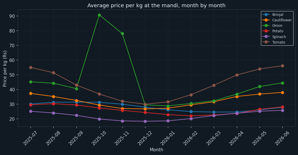
One line per vegetable, month by month. Six lines on one pair of axes is close to the limit of what a reader can follow, and it is worth it here because the comparison between the lines is the whole point.
Five of the six lines are gentle waves. Potato runs between Rs 22 and Rs 30 all year, brinjal between Rs 24 and Rs 31, spinach between Rs 18 and Rs 26. Tomato swings harder, from Rs 29.88 in December to Rs 56.09 in June.
Then there is the onion, which leaves the group entirely in October and November and comes back down in December. Everything else on this chart is a season; that is an event. Putting all six on one chart is what makes the difference obvious — on six separate charts the onion would just look like another line with a bump in it.
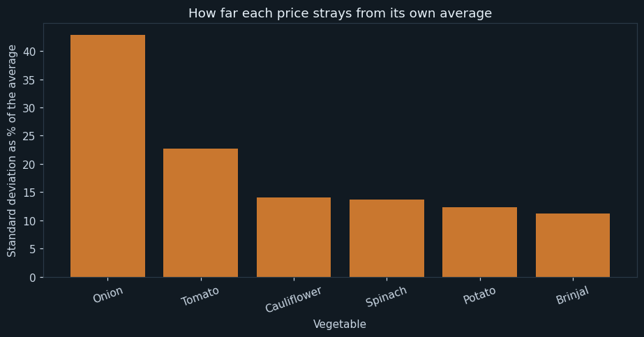
For each vegetable, how far its price typically strays from its own average, as a percentage. Using a percentage rather than rupees is what lets a Rs 18 vegetable be compared with a Rs 45 one.
Onion strays 42.8 per cent from its own average and tomato 22.7. Brinjal strays 11.2, potato 12.3 and spinach 13.7.
That splits the six into two groups with a real gap between them. Four vegetables are budgetable: whatever they cost this week, they will cost roughly that next month. Two are not, and one of those is the vegetable that goes into almost every Indian meal. A household that knows this buys onions differently from the way it buys potatoes — in more quantity when they are cheap, and without assuming this week's price says anything about next month's.
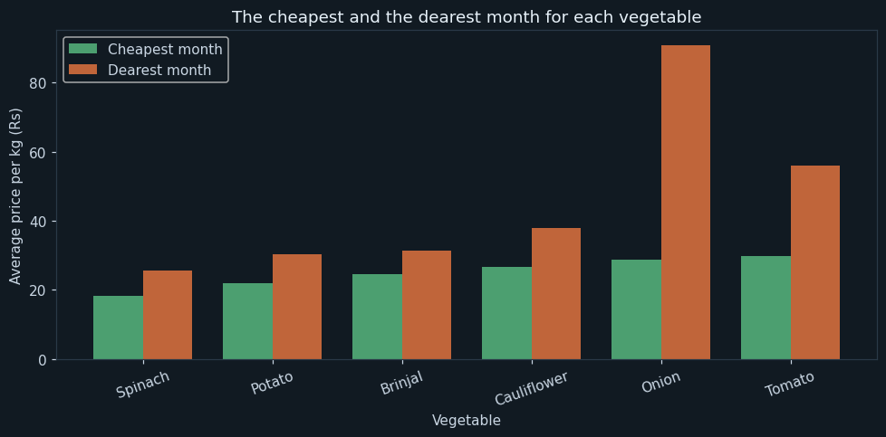
Two bars for each vegetable: its average in its cheapest month and in its dearest. Side by side, so the gap between the pair is what the eye reads.
For four of the six the two bars are close: potato ranges 1.4 times from its cheapest month to its dearest, brinjal 1.3, spinach 1.4, cauliflower 1.4. Tomato is 1.9.
Onion is 3.2 times — Rs 28.75 in January against Rs 90.74 in October. It is also worth reading the cheap months as a group: cauliflower, spinach and tomato are all cheapest in December, which is simply the north Indian winter crop arriving. That is the month to buy and preserve, and it is the same month for three different vegetables.
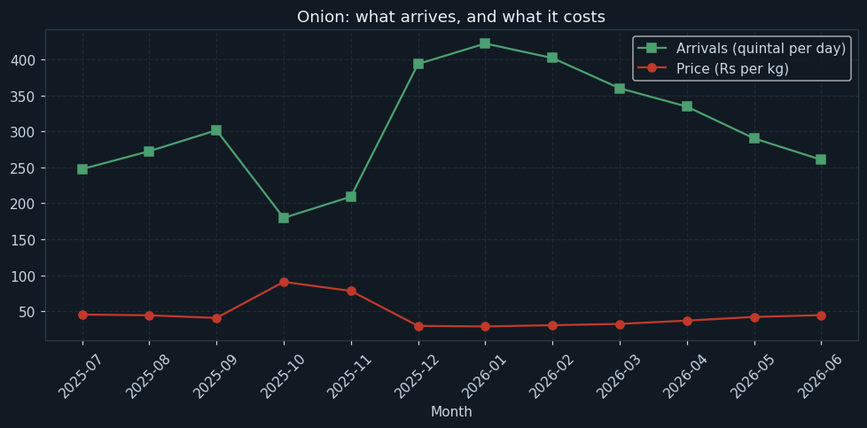
Two lines for the onion alone: the average daily arrivals in quintals, and the average price per kilogram, month by month. Two quantities in different units on one chart, which works here because it is the shape of the two lines against each other that matters, not their heights.
The two lines are almost exact mirrors. Arrivals fall from 302 quintals a day in September to 180 in October; the price goes from Rs 40.52 to Rs 90.74. In December arrivals recover to 394 and the price drops to Rs 29.44.
This is the chart that answers the argument. The onion did not become expensive because somebody decided it should — 40 per cent less of it turned up. And the recovery is just as sharp: as soon as the new crop arrived the price collapsed back to normal within a month.
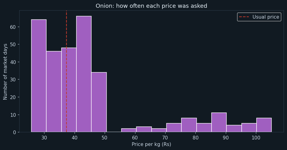
Every market day's onion price sorted into sixteen bands, with a dashed line at the usual price — the average of the ten months that were not the spike. A histogram, because the question is how the year's days were distributed.
The bulk of the year sits in a hump between about Rs 26 and Rs 50, and then there is a long thin scatter of days out to Rs 105.13, the dearest day of the year, on 6 October.
In a normal month onion averaged Rs 37.37; across October and November it averaged Rs 84.40, which is 2.26 times the usual price. And the tail is thin — those two months are about a sixth of the year's market days. Most of the year the onion was ordinary, which is exactly the part nobody remembers.
12What the analysis found
- Onion strays 42.8 per cent from its own average; brinjal strays 11.2.
- Onion cost 3.2 times as much in its dearest month as in its cheapest — Rs 90.74 against Rs 28.75.
- The October–November onion price averaged Rs 84.40 against a usual Rs 37.37 — 2.26 times.
- The dearest single day was Rs 105.13 a kilogram on 6 October.
- Onion arrivals fell from 302 quintals a day in September to 180 in October, and recovered to 394 by December.
- Price and arrivals are negatively correlated for all six vegetables, from -0.455 for brinjal to -0.798 for tomato.
- Cauliflower, spinach and tomato are all at their cheapest in December.
What should be done about them
This is the part that turns an analysis into a project. A chart that nobody acts on is a picture; a recommendation somebody can argue with is a result.
- Buy onions in quantity in December and January, when they are at their cheapest and the new crop is in.
- Budget potato, brinjal, spinach and cauliflower at their average; they will not surprise you.
- Do not budget onion or tomato at their average. Either allow for the spike or buy them differently.
- December is the month to buy and preserve. Three of the six are at their lowest in it.
- Keep copying the board. One year shows the pattern; three years would show whether it repeats, which is the question that actually matters.
13Testing
Every case below was actually executed and its result recorded as it appeared — including the ones expected to fail. Each one builds a small dataset of its own and runs the whole program against it.
| Test case | Expected | Actual | Result |
|---|---|---|---|
| The full board, 1873 rows | Entries used : 1867 | Entries used : 1867 | Pass |
| Days the board was not noted are dropped | Days the board was not noted: 5 (dropped) | Days the board was not noted: 5 (dropped) | Pass |
| A day copied twice is removed | Duplicate entries : 1 | Duplicate entries : 1 | Pass |
| Two spellings fold into six vegetables, not eight | Vegetables : ['Brinjal', 'Cauliflower', 'Onion', 'Potato', 'Spinach', 'Tomato'] | Vegetables : ['Brinjal', 'Cauliflower', 'Onion', 'Potato', 'Spinach', 'Tomato'] | Pass |
| The two dearest months are found in the data, not written into the code | Dearest two months : 2025-10, 2025-11 | Dearest two months : 2025-10, 2025-11 | Pass |
| The onion spike measured against the usual price | The spike was 2.26 times the usual price. | The spike was 2.26 times the usual price. | Pass |
| A price that never changes strays 0.0 per cent from its average | Potato 20.0 0.0 20.0 20.0 0.0 | Potato 20.0 0.0 20.0 20.0 0.0 | Pass |
| Prices of 10 and 30 give a swing of 70.7 per cent | Potato 20.0 14.14 10.0 30.0 70.7 | Potato 20.0 14.14 10.0 30.0 70.7 | Pass |
| A cheap vegetable and a dear one with the same swing rank equally | Tomato 200.0 141.42 100.0 300.0 70.7 | Tomato 200.0 141.42 100.0 300.0 70.7 | Pass |
| A price that falls exactly as arrivals rise correlates at -1.0 | Potato correlation between price and arrivals: -1.000 | Potato correlation between price and arrivals: -1.000 | Pass |
| "onion" and "Onion" are counted as one vegetable | Vegetables : ['Onion'] | Vegetables : ['Onion'] | Pass |
| mandi.csv missing altogether | FileNotFoundError: [Errno 2] No such file or directory: 'mandi.csv' | FileNotFoundError: [Errno 2] No such file or directory: 'mandi.csv' | Pass |
Two kinds of case are in there on purpose. The boundary cases test the edge of a rule, where a program is most often wrong by one. The failure cases check that it stops cleanly and says why, instead of quietly producing a wrong answer.
14Advantages
Set against the ways the job is done today:
- It replaces remembered prices, which are systematically too high, with recorded ones
- Vegetables of very different prices are compared fairly, using the swing as a percentage
- Price and arrivals are set side by side, which is what turns a complaint into an explanation
- The data can genuinely be collected by one person in two minutes a day
- Adding next year's board changes nothing in the program
15Limitations and future scope
What this version cannot tell you
A data project should be honest about the limits of its own data. Each of these is a reason for one of the additions below:
- Mandi prices, not shop prices — what a household pays includes the retailer's margin on top
- Six vegetables out of the dozens a mandi handles
- One market and one year, so nothing here says whether the pattern repeats
- Quality is not recorded, and a price is for whatever grade was on the board that day
- Correlation is not cause: low arrivals and high prices moving together does not prove which produced which, though in a market the direction is not really in doubt
What to add next
This is also where you make the project yours. Take one or two of these, or something nobody here thought of:
- Collect a second year and put the two on one chart to see whether the onion spike is annual
- Add the retail price from a local shop and chart the margin between the two
- Pull the figures from Agmarknet automatically instead of copying them
- Add more vegetables, and pulses, which behave differently again
- Work out what a fixed weekly vegetable basket would have cost each month across the year
- Compare against the rainfall data from the weather project, and see whether a bad monsoon shows up in the prices
16What you may have to teach yourself
CBSE expects some self-learning in a project and says so. For this one, that means:
- Standard deviation, and why dividing it by the mean is what makes two different price levels comparable. This is the one statistical idea in the project and it is worth understanding rather than copying.
- pivot_table(), which turns a long thin file into the wide table a multi-line chart needs
- Why to_period("M") produces YYYY-MM and why that format sorts correctly when "March" does not
- Where real mandi data lives — Agmarknet and your state's agricultural marketing board — and how to cite it
17Conclusion
The program does what it set out to do. A year of a public price board, copied down in two minutes a day, comes back as five charts and a month-by-vegetable table, and the questions a household argues about have figures behind them.
The finding that changes how somebody shops is the second chart, not the onion. Four of these six vegetables move barely more than ten per cent from their own average all year, and two move two to four times that. Nobody at a vegetable stall knows which group they are in, because a single week's price looks the same either way. Knowing it is the difference between a budget that works and one that is broken twice a year.
The onion is the more satisfying result because it is a complete story in one file. Arrivals fell by 40 per cent, the price went to 2.26 times normal for two months, the new crop came in and the price collapsed back inside a month. Everybody in the country had an opinion about that October. The price board had the answer posted on it the whole time, and it cost two minutes a day to write down. The program does not name October anywhere: it finds the two dearest months itself, which is what lets the same code be run on next year's board.
18References
Every report needs a bibliography, and a data project needs its data source at the top of it.
- The public price board of a vegetable mandi, one year. The dataset shipped here is a LambdaLab sample standing in for it and is not a record of any real market.
- Agmarknet, Directorate of Marketing and Inspection — https://agmarknet.gov.in/
- pandas user guide, “Reshaping and pivot tables” — https://pandas.pydata.org/docs/user_guide/reshaping.html
- Informatics Practices, Class XII — the NCERT / CBSE prescribed textbook, for the chapters on data handling with pandas and data visualisation
- pandas documentation — https://pandas.pydata.org/docs/
- Matplotlib documentation — https://matplotlib.org/stable/
- CBSE Senior School Curriculum, Informatics Practices (Subject Code 065) — the project guidelines this report follows
- LambdaLab — https://www.lambdalab.in