Reading a Class XII Result
Seventy students, five subjects, three terms — and the questions a mark register can answer but never does.
1Introduction: the problem it solves
Every school keeps a mark register. Marks go in three times a year, a percentage is worked out for each student, and the register is put away. At the result meeting somebody says the class is weak in Physics, somebody else disagrees, and neither of them has looked.
The register can settle it. It holds every mark of every student in every subject in every term, which is more than enough to say which subject is weakest, whether the class is improving, how the grades are spread, whether one section is ahead of the other, and exactly which students need help before the board examination.
Nobody works those out, because doing it by hand for 1,050 marks is a day's work that has to be repeated every term. Done in pandas it takes a second, and it can be repeated the day the marks are entered.
A class teacher, a head of department, or the school's examination in-charge — anybody who has to stand up at the result meeting and say something useful.
Why it is worth doing on a computer
A result is only useful while there is still time to act on it. Working out by hand which students are at risk takes long enough that the answer arrives after the extra classes would have had to start. Speed is not a convenience here — it is the difference between a report and an intervention.
There is a second reason, which matters more. Doing this by hand, a teacher looks at the marks they already suspect are a problem. A program looks at all of them, including the section that quietly slipped, the subject that improved most and the student whose one weak subject is hidden by a decent average. Those are exactly the findings a human eye skips, and they are in the register the whole time.
Objectives
- To read a whole class's mark register out of one CSV file, in the shape the marks are already entered in
- To handle an absent student honestly, so an absence never becomes a zero
- To find the class's weakest and strongest subjects in the final examination
- To show whether the class improved between Term 1 and the Final, subject by subject
- To produce the CBSE grade distribution and the spread of percentages across the class
- To compare the two sections subject by subject, and say by how much they differ
- To name every student below the pass mark, and rank the ten lowest for extra classes
2How the job is done today
Before writing anything it is worth asking how the work is handled at present, and where each of those answers falls short. These were examined:
Complete and authoritative, and answers nothing on its own. Every question above means reading it row by row with a calculator, so those questions get asked once a year at most.
What most schools have moved to, and a real improvement. Averages and grades are easy; comparing three terms, two sections and five subjects at once means building the same set of formulas again every term, and that is where the mistakes live.
Prints report cards well. The analysis it offers is whatever its makers put in, it usually stops at averages, and getting the raw marks back out of it to ask a different question is often impossible.
Valuable and not to be dismissed — but it is formed from the students a teacher notices. The section difference this project found is 1.5 to 2.5 marks, which is real and is far too small for anyone to have felt.
3Where the data came from
CBSE asks that any resource used in a project be suitably referenced, and for a data project that rule is not a formality — a figure with no source attached to it does not mean anything. This section is the one an examiner will ask about.
The marks come from the school's own register, entered as one row per student per subject per term. That shape is deliberate: it is how marks are actually written down, so nothing has to be rearranged before typing, and adding a fourth term later means adding rows rather than redesigning the file.
There is not a single name in the file. Students are identified by roll number, and that decision came before any data was copied. A result analysis gets shown in staff meetings and pinned to notice boards, and it has no business carrying children's names attached to their marks.
The dataset here is a LambdaLab sample of 1,050 rows, built to behave like a real register including the gaps. Use your own school's marks in your submission, get the examination in-charge's permission first, keep the roll numbers and leave the names out.
4The dataset
One file in, one file out. results.csv holds one mark per row — student, section, subject, term, marks. Long and thin like this is easier to type and far easier to filter than a wide sheet with fifteen columns; pivot_table turns it into whatever wide shape a chart needs.
results.csv — one row per student per subject per term
| Field | Type | What it holds |
|---|---|---|
roll_no | text | The student's roll number, e.g. 12A25. Section is in it, and no name is. |
section | text | A or B. |
subject | text | English, Physics, Chemistry, Mathematics or Computer Science. |
term | text | Term 1, Term 2 or Final. |
marks | integer | Marks out of 100. Blank if the student was absent for that test. |
The first few lines of results.csv
| roll_no | section | subject | term | marks |
|---|---|---|---|---|
12A25 | A | Chemistry | Term 1 | 63 |
12B25 | B | English | Final | 99 |
12B24 | B | English | Term 2 | 99 |
12A29 | A | Mathematics | Final | 63 |
12A25 | A | English | Final | 72 |
12B25 | B | Physics | Term 2 | 72 |
12B01 | B | Physics | Term 2 | 70 |
12A35 | A | Mathematics | Term 2 | 57 |
Inside results.csv
The mark register: 1,050 rows covering 70 students, 5 subjects and 3 terms, with six absences left blank exactly as they are in the register. The whole file is 1,050 rows, 29.4 KB — too much to print here, so this is the head of it. The complete file comes with the download, and you can also take it on its own.
roll_no,section,subject,term,marks
12A25,A,Chemistry,Term 1,63
12B25,B,English,Final,99
12B24,B,English,Term 2,99
12A29,A,Mathematics,Final,63
12A25,A,English,Final,72
12B25,B,Physics,Term 2,72
12B01,B,Physics,Term 2,70
12A35,A,Mathematics,Term 2,575Cleaning the data
Real data arrives with mistakes in it, and this dataset has the ones real data actually has. What was wrong, how much of it there was, and what the program does about each — because how a problem is handled changes the answer, and a report has to say which choice it made.
The row is dropped and the count printed. This is the most important decision in the project: an absence is not a zero, and averaging it as one would drag the subject average down and make every figure that follows wrong.
While a blank is present pandas has to store the column as float, so 63 reads as 63.0. astype(int) after the blanks are gone puts it back to whole marks.
str.strip().str.title() folds them back. The register is typed by more than one person, and the program printed 7 subjects before this line and 5 after it — which is exactly how the problem was noticed.
"Final" comes before "Term 1" in the alphabet, so a chart drawn without reindex(["Term 1", "Term 2", "Final"]) shows the year running backwards and looks like a class that got worse.
6What the program does
- Reads a whole class's mark register from one CSV file
- Drops absences without letting them become zeros, and reports how many there were
- Ranks the five subjects by their average in the final examination, against the pass mark
- Tracks every subject across Term 1, Term 2 and the Final, and prints how much each moved
- Works out each student's percentage and turns it into a CBSE grade band
- Counts the grade distribution and draws the spread of percentages
- Compares Section A with Section B subject by subject and prints the difference
- Names every failing entry in the final, and ranks the ten lowest students for extra classes
- Writes the whole ranking out as a CSV the class teacher can sort
The pandas and pyplot it is built from
| Call | Where | What it is for |
|---|---|---|
pd.read_csv() | step 1 | Loads the register |
Series.isnull().sum() | step 2 | Counts the absences before anything is dropped |
df.dropna(subset=["marks"]) | step 2 | Removes the absences only |
Series.astype(int) | step 2 | Puts marks back to whole numbers once the blanks are gone |
Series.str.strip().str.title() | step 2 | Folds "PHYSICS" back into "Physics" |
df[df["term"] == "Final"] | step 3 | Boolean indexing — keeps the rows that answer this question |
df.groupby(col)[v].mean() | steps 4–6 | The subject averages and each student's percentage |
df.pivot_table(index=, columns=) | steps 4, 6 | Terms against subjects, and subjects against sections |
DataFrame.reindex([...]) | steps 4, 5 | Forces Term 1, Term 2, Final into that order, not alphabetical |
Series.apply(function) | step 5 | Runs grade() on every percentage in the column |
Series.value_counts() | step 5 | How many students in each grade band |
Series.idxmin() / idxmax() | steps 3, 5 | Which subject is weakest, which student is top |
plt.axhline() | chart 1 | The red line marking the pass mark across the chart |
plt.bar(x - w/2) and plt.bar(x + w/2) | chart 5 | Two sets of bars side by side, one per section |
DataFrame.to_csv() | step 7 | Writes the ranked list out for the class teacher |
7Technical details
| Language | Python 3 |
| Where the data lives | A plain CSV file, read into pandas |
| Libraries |
|
8How it works, step by step
read_csv() loads results.csv — 1,050 rows, one mark each.
Absences are dropped and counted, the marks column is put back to whole numbers, and subject spellings are folded together.
df[df["term"] == "Final"] keeps only the final examination for the questions that are about the final. Boolean indexing, and nothing more complicated.
groupby() gives the subject averages and each student's percentage. pivot_table() lays terms against subjects, and subjects against sections, which is the shape the charts need.
A small grade() function turns a percentage into a CBSE band, and apply() runs it down the whole column.
Five charts — a bar, a multi-line, a bar, a histogram and a pair of side-by-side bars — each saved with savefig().
9Source code
The whole program. Every chart further down this page was drawn by this listing, and every figure quoted came out of running it.
# ---------------------------------------------------------------------------
# result_analysis.py
#
# Reads the mark register of two Class XII sections from results.csv and
# answers what the class teacher has to say at the result meeting:
#
#   1. Which subject is the class weakest in?
#   2. Is the class improving from Term 1 to the Final, or drifting?
#   3. How are the grades spread — a few toppers, or a solid middle?
#   4. Is one section doing better than the other, and in which subject?
#   5. Which students need help before the board examination?
#
# The register is one row per student per subject per term, which is how the
# marks are entered. Everything below is built from that one shape.
# ---------------------------------------------------------------------------

import pandas as pd
import matplotlib.pyplot as plt

PASS_MARK = 33          # CBSE pass mark in a subject

# --- 1. Read -------------------------------------------------------------
df = pd.read_csv("results.csv")

print("Rows read      :", len(df))
print("Students       :", df["roll_no"].nunique())
print("Subjects       :", df["subject"].nunique())
print()

# --- 2. Clean ------------------------------------------------------------
# A blank marks cell means the student was absent for that test. An absence is
# not a zero — averaging it as zero would drag the subject average down and
# make the whole report wrong — so those rows are dropped and counted.
absent = df["marks"].isnull().sum()
df = df.dropna(subset=["marks"])
df["marks"] = df["marks"].astype(int)      # the column was float while NaN was in it

# The register was typed by more than one person, so a subject appears in
# capitals here and there. str.title() makes them one subject again.
df["subject"] = df["subject"].str.strip().str.title()

print("Absent entries dropped :", absent)
print("Subjects after tidying :", sorted(df["subject"].unique()))
print()

# --- 3. Question 1: which subject is the class weakest in? ---------------
# The Final is what matters for this question, so the other two terms are
# filtered out first with a boolean condition.
final = df[df["term"] == "Final"]

subject_avg = final.groupby("subject")["marks"].mean().sort_values()
print("--- Final: average marks by subject ---")
print(subject_avg.round(1))
print()
print("Weakest subject:", subject_avg.idxmin(), "at", round(subject_avg.min(), 1))
print()

plt.figure(figsize=(8, 4.5))
plt.bar(subject_avg.index, subject_avg.values, color="#3b7dd8")
plt.axhline(PASS_MARK, color="#c0392b", linestyle="--", label="Pass mark (33)")
plt.title("Final examination: average marks by subject")
plt.xlabel("Subject")
plt.ylabel("Average marks out of 100")
plt.xticks(rotation=20)
plt.legend()
plt.tight_layout()
plt.savefig("chart1_subject_average.png")
plt.close()

# --- 4. Question 2: is the class improving? ------------------------------
# pivot_table puts terms across the top and subjects down the side, which is
# the shape a multi-line chart wants: one line per subject.
trend = df.pivot_table(index="term", columns="subject", values="marks", aggfunc="mean")

# "Final" comes before "Term 1" in the alphabet, so without this line the
# chart would show the year running backwards and a class that improved would
# look like one that slipped. Only the terms actually in the file are kept,
# so a register holding just the final still works.
wanted = ["Term 1", "Term 2", "Final"]
trend = trend.reindex([t for t in wanted if t in trend.index])

print("--- Average marks, term by term ---")
print(trend.round(1))
print()
if "Term 1" in trend.index and "Final" in trend.index:
    print("Change from Term 1 to Final:")
    print((trend.loc["Final"] - trend.loc["Term 1"]).round(1))
else:
    print("Only one term is in the file, so there is no change to report.")
print()

plt.figure(figsize=(9, 4.5))
for subject in trend.columns:
    plt.plot(trend.index, trend[subject], marker="o", label=subject)
plt.title("Average marks, Term 1 to Final")
plt.xlabel("Term")
plt.ylabel("Average marks")
plt.legend(fontsize=8)
plt.grid(True, linestyle="--", alpha=0.5)
plt.tight_layout()
plt.savefig("chart2_term_trend.png")
plt.close()

# --- 5. Question 3: how are the grades spread? ---------------------------
# Each student's percentage in the Final is the mean of their five subjects.
percent = final.groupby("roll_no")["marks"].mean().round(1)

def grade(p):
    """The CBSE grade band a percentage falls into."""
    if p >= 91: return "A1"
    if p >= 81: return "A2"
    if p >= 71: return "B1"
    if p >= 61: return "B2"
    if p >= 51: return "C1"
    if p >= 41: return "C2"
    if p >= 33: return "D"
    return "E"

# apply() runs grade() on every value of the Series and gives a Series back.
grades = percent.apply(grade)
bands = ["A1", "A2", "B1", "B2", "C1", "C2", "D", "E"]
counts = grades.value_counts().reindex(bands).fillna(0).astype(int)

print("--- Grade distribution (Final) ---")
print(counts)
print()
print("Class percentage : ", round(percent.mean(), 1))
print("Highest          : ", percent.max(), "(", percent.idxmax(), ")")
print("Lowest           : ", percent.min(), "(", percent.idxmin(), ")")
print()

plt.figure(figsize=(8, 4.5))
plt.bar(counts.index, counts.values, color="#4c9f70")
plt.title("Grade distribution in the Final examination")
plt.xlabel("Grade")
plt.ylabel("Number of students")
plt.tight_layout()
plt.savefig("chart3_grades.png")
plt.close()

plt.figure(figsize=(8, 4.5))
plt.hist(percent.values, bins=10, color="#a05fc0", edgecolor="white")
plt.title("Spread of final percentages")
plt.xlabel("Percentage")
plt.ylabel("Number of students")
plt.tight_layout()
plt.savefig("chart4_percent_spread.png")
plt.close()

# --- 6. Question 4: is one section ahead? --------------------------------
by_section = final.pivot_table(index="subject", columns="section",
                               values="marks", aggfunc="mean").round(1)

# The sections are read out of the file rather than written into the program,
# so a school with three sections — or one — needs no change here. The
# difference column only makes sense when there are exactly two.
sections = list(by_section.columns)
if len(sections) == 2:
    by_section["Difference"] = (by_section[sections[0]] - by_section[sections[1]]).round(1)

print("--- Section %s against Section %s (Final) ---" % (sections[0], sections[-1]))
print(by_section)
print()

plt.figure(figsize=(9, 4.5))
x = range(len(by_section.index))
width = 0.8 / len(sections)
colours = ["#3b7dd8", "#e07b39", "#4c9f70"]
# One set of bars per section, each shifted a little so they sit side by side
# at every subject. That shift is the whole trick to a grouped bar chart.
for n, sec in enumerate(sections):
    offset = (n - (len(sections) - 1) / 2) * width
    plt.bar([i + offset for i in x], by_section[sec], width,
            label="Section " + sec, color=colours[n % len(colours)])
plt.xticks(list(x), by_section.index, rotation=20)
plt.title("The sections compared, subject by subject")
plt.xlabel("Subject")
plt.ylabel("Average marks")
plt.legend()
plt.tight_layout()
plt.savefig("chart5_sections.png")
plt.close()

# --- 7. Question 5: who needs help? --------------------------------------
# A student is flagged if any subject in the Final is below the pass mark.
weak = final[final["marks"] < PASS_MARK]
print("--- Failing entries in the Final ---")
if len(weak) == 0:
    print("None. No student is below", PASS_MARK, "in any subject.")
else:
    print(weak[["roll_no", "subject", "marks"]].to_string(index=False))
print()

# The bottom of the class, whether or not anyone has actually failed.
print("--- Ten lowest percentages, for extra classes ---")
print(percent.sort_values().head(10))
print()

percent.sort_values().to_csv("students_ranked.csv", header=["percent"])
print("Charts saved : chart1_subject_average.png .. chart5_sections.png")
print("Ranking saved: students_ranked.csv")The full report as a PDF, ready to print and fill in. Or the working project as a zip — the program, the dataset, the charts and a README.
10Sample output
A real run, reproduced exactly as it appeared. Nothing below was typed by hand — it is the transcript of the program above against the dataset in section 4.
Rows read      : 1050
Students       : 70
Subjects       : 7

Absent entries dropped : 6
Subjects after tidying : ['Chemistry', 'Computer Science', 'English', 'Mathematics', 'Physics']

--- Final: average marks by subject ---
subject
Physics             62.7
Mathematics         63.9
Chemistry           66.4
Computer Science    73.2
English             76.4
Name: marks, dtype: float64

Weakest subject: Physics at 62.7

--- Average marks, term by term ---
subject  Chemistry  Computer Science  English  Mathematics  Physics
term
Term 1        61.9              66.0     71.4         60.0     56.4
Term 2        63.5              70.2     72.4         61.9     59.0
Final         66.4              73.2     76.4         63.9     62.7

Change from Term 1 to Final:
subject
Chemistry           4.5
Computer Science    7.2
English             5.0
Mathematics         4.0
Physics             6.3
dtype: float64

--- Grade distribution (Final) ---
marks
A1     2
A2    13
B1    12
B2    23
C1    16
C2     3
D      1
E      0
Name: count, dtype: int64

Class percentage :  68.5
Highest          :  98.2 ( 12B24 )
Lowest           :  36.8 ( 12A18 )

--- Section A against Section B (Final) ---
section              A     B  Difference
subject
Chemistry         65.3  67.5        -2.2
Computer Science  72.0  74.5        -2.5
English           75.6  77.1        -1.5
Mathematics       63.8  64.1        -0.3
Physics           62.5  62.9        -0.4

--- Failing entries in the Final ---
roll_no     subject  marks
  12A18     Physics     19
  12A19     Physics     29
  12A18 Mathematics     31

--- Ten lowest percentages, for extra classes ---
roll_no
12A18    36.8
12A19    46.2
12A20    49.6
12B31    50.2
12B02    51.8
12A14    53.6
12B26    54.2
12B16    54.6
12B32    55.2
12B14    55.2
Name: marks, dtype: float64

Charts saved : chart1_subject_average.png .. chart5_sections.png
Ranking saved: students_ranked.csv
Running it also wrote students_ranked.csv — 70 rows. This is the head of it:
roll_no,percent
12A18,36.8
12A19,46.2
12A20,49.6
12B31,50.2
12B02,51.8
12A14,53.6
12B26,54.2
12B16,54.6
12B32,55.211The charts, and what each one says
CBSE asks for appropriate charts, and the word doing the work in that phrase is appropriate. A line for something that moves in order, a bar to compare things that do not, a histogram for the shape of one column of numbers. Each chart below says which it is, why that kind was chosen, and what it turned out to show.
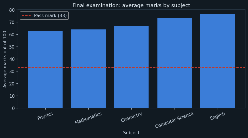
One bar per subject in the final examination, weakest on the left, with a dashed red line at the pass mark of 33. Bars, because five subjects have no natural order and the point is to compare heights.
Physics is the weakest subject at 62.7 and English the strongest at 76.4 — a gap of 13.7 marks between the two ends of the same class's report card.
The pass line is worth leaving on the chart even though every bar clears it easily. It is the reminder that this chart is about averages: a subject can average 62.7 and still have students at 19, and the last section of the program is what finds them.
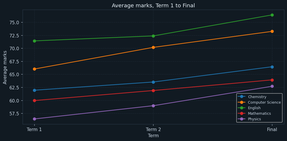
Five lines, one per subject, across Term 1, Term 2 and the Final. A line chart because the three terms are in order and the shape of the movement is the whole point.
Every one of the five lines goes up. The class improved in all five subjects, by between 4.0 and 7.2 marks, and Computer Science improved most.
Physics is the interesting one: it gained 6.3 marks, the second-largest improvement of any subject, and it is still bottom of the class. Those two facts together say something the first chart could not — the teaching is working and the subject started further back. "Weak in Physics" and "getting worse at Physics" are different claims, and only one of them is true here.
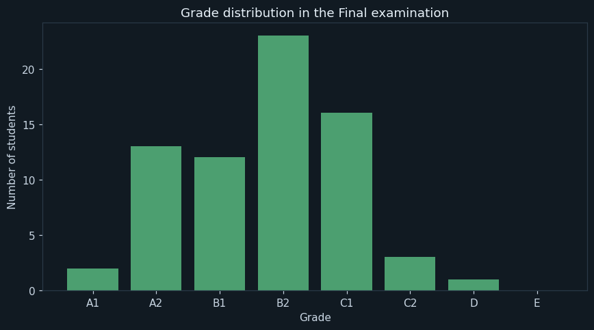
The eight CBSE grade bands from A1 to E, with the number of students in each. The bands are in order, so the bars can be read left to right like a scale.
The class is a hump in the middle: B2 is the largest band with 23 students, then C1 with 16, A2 with 13 and B1 with 12. Two students take A1 and one is in D.
There is nobody in E, which means no student is below 33 per cent overall. That is not the same as nobody failing — three individual subject entries are below the pass mark, and they belong to two students whose other subjects carry their average up. A grade distribution can hide a failing subject completely, which is why the program prints the failing entries separately.
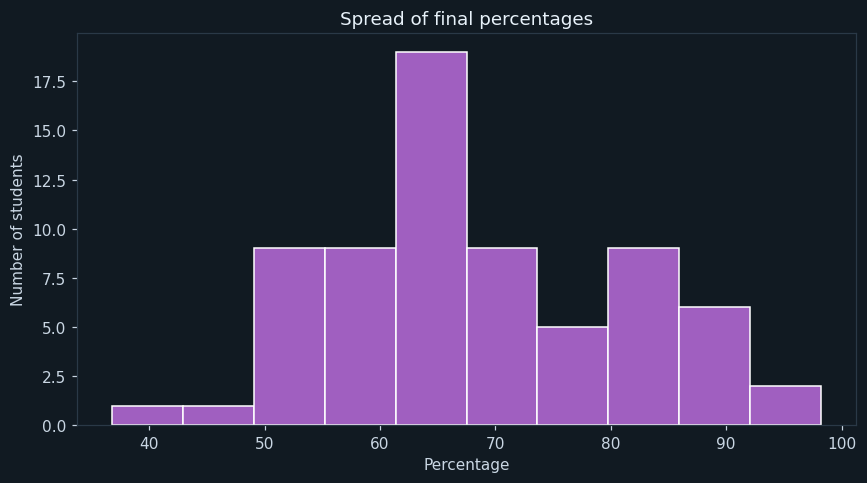
The 70 students' final percentages sorted into ten bands, with the height of each bar showing how many landed in it. A histogram is for one column of numbers where the question is the shape, not the individuals.
The class average is 68.5, the top is 98.2 and the bottom 36.8 — a spread of over 61 percentage points inside one class taught by the same teachers.
The shape is a broad hump with a thin tail to the left. That tail is small enough to do something about: it is the four or five students who need extra classes, and this chart is what tells a head of department that helping them is a small job, not a hopeless one.
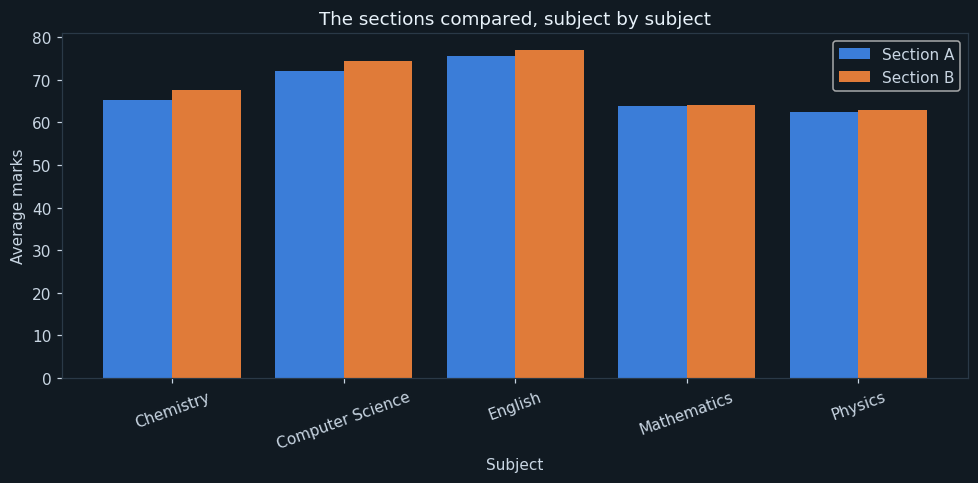
Two bars at each subject, one per section, drawn side by side so the pair can be compared directly. This is the chart to use whenever two groups are being set against each other.
Section B is ahead in all five subjects, by between 0.3 and 2.5 marks. The largest gaps are Computer Science at 2.5 and Chemistry at 2.2; Mathematics and Physics are within half a mark and are effectively level.
The honest reading is the modest one. A consistent lead of one to two marks across five subjects is worth noticing, but it is small, it is one year, and nothing here says why. It is a reason to ask a question at the next department meeting, not a finding to announce.
12What the analysis found
- The class averages 68.5 per cent in the final, spread from 36.8 to 98.2.
- Physics is weakest at 62.7 and English strongest at 76.4 — a gap of 13.7 marks.
- All five subjects improved from Term 1 to the Final, by 4.0 to 7.2 marks.
- B2 is the biggest grade band with 23 of 70 students; two take A1 and none is in E.
- Section B leads Section A in every subject, but only by 0.3 to 2.5 marks.
- Three subject entries are below the pass mark, and they belong to two students.
- Six of the 1,050 entries are absences, and treating them as zero would have moved every average.
What should be done about them
This is the part that turns an analysis into a project. A chart that nobody acts on is a picture; a recommendation somebody can argue with is a result.
- Start extra Physics classes with the four students at the bottom of the ranked list, not with the whole class.
- Look at 12A18 and 12A19 individually — both have a failing entry hidden behind a passing average.
- Whatever changed in Computer Science between Term 1 and the Final is worth asking the department about; it is the largest gain of the year.
- Do not act on the section difference yet. Run this again next year before deciding it is real.
- Chase the six absences. A test not sat is a data point missing from every figure in this report.
13Testing
Every case below was actually executed and its result recorded as it appeared — including the ones expected to fail. Each one builds a small dataset of its own and runs the whole program against it.
| Test case | Expected | Actual | Result |
|---|---|---|---|
| The full register, 1050 rows | Class percentage : 68.5 | Class percentage : 68.5 | Pass |
| Absences found and dropped | Absent entries dropped : 6 | Absent entries dropped : 6 | Pass |
| Two spellings of a subject folded into one | Subjects after tidying : ['Chemistry', 'Computer Science', 'English', 'Mathematics', 'Physics'] | Subjects after tidying : ['Chemistry', 'Computer Science', 'English', 'Mathematics', 'Physics'] | Pass |
| An absence is left out, not counted as zero | Class percentage : 80.0 | Class percentage : 80.0 | Pass |
| A student on exactly 91 per cent is graded A1 | A1 1 | A1 1 | Pass |
| A student on exactly 90 per cent is graded A2 | A2 1 | A2 1 | Pass |
| A student on exactly 33 per cent is graded D | D 1 | D 1 | Pass |
| A student on exactly 32 per cent is graded E | E 1 | E 1 | Pass |
| 33 in a subject is a pass, not a failure | None. No student is below 33 in any subject. | None. No student is below 33 in any subject. | Pass |
| 32 in a subject is picked up as a failure | 12A01 English 32 | 12A01 English 32 | Pass |
| The three terms come out in the right order | Term 1 40.0 40.0 40.0 40.0 40.0 | Term 1 40.0 40.0 40.0 40.0 40.0 | Pass |
| results.csv missing altogether | FileNotFoundError: [Errno 2] No such file or directory: 'results.csv' | FileNotFoundError: [Errno 2] No such file or directory: 'results.csv' | Pass |
Two kinds of case are in there on purpose. The boundary cases test the edge of a rule, where a program is most often wrong by one. The failure cases check that it stops cleanly and says why, instead of quietly producing a wrong answer.
14Advantages
Set against the ways the job is done today:
- The register is analysed the day the marks go in, while there is still time to act
- Every subject, section and term is examined, not just the ones somebody already suspects
- Absences are handled correctly and reported, instead of quietly becoming zeros
- Grade bands are applied by a rule in one place, so nobody has to remember where A2 starts
- The comparisons come with their sizes attached, which stops a two-mark gap being talked about as a crisis
- Running it again next term is one command, so the trend actually gets built
15Limitations and future scope
What this version cannot tell you
A data project should be honest about the limits of its own data. Each of these is a reason for one of the additions below:
- It reports marks and nothing else — attendance, effort and circumstances are not in the file
- One year of one class; a trend needs several
- The grade bands are the simple CBSE percentage bands, not the board's own statistical grading
- It cannot say why anything happened, only what did
- Sections are compared as they stand, with no allowance for how students were placed in them
What to add next
This is also where you make the project yours. Take one or two of these, or something nobody here thought of:
- Add attendance as a column and see whether it tracks the marks
- Read several years and chart a subject's average across them
- Print a one-page sheet per student with their five subjects and their three terms
- Flag any student whose marks fell in two subjects at once, which is the pattern worth catching early
- Let a teacher pick the subject and the term from the keyboard instead of editing the code
- Compare against the board's published subject averages, where they are available
16What you may have to teach yourself
CBSE expects some self-learning in a project and says so. For this one, that means:
- pivot_table() — the one idea in this project worth real practice. index, columns and aggfunc between them turn a long thin file into any table you need.
- reindex() and why a chart of terms comes out backwards without it
- apply() with a function of your own, which is how the grade bands are done
- How your school's grading actually works — school grade bands and CBSE board grading are not the same thing, and your report should say which it uses
17Conclusion
The program does what it set out to do. A mark register that answers nothing on its own now answers seven questions in about a second, and the same command will answer them again next term.
The result worth keeping is a pair of findings that contradict the obvious one. Physics is the weakest subject in the class and it is also the second most improved — so the register does not support the sentence people were saying at the result meeting. And the grade distribution, which looks entirely healthy with nobody in E, hides two students who are failing a subject each.
Writing it made one decision matter more than all the rest: what to do with six blank cells. Treating an absence as a zero would have been one word shorter to write and would have moved every average in the report. Most of the work in a data project is that kind of decision, not the charts.
18References
Every report needs a bibliography, and a data project needs its data source at the top of it.
- The Class XII mark register of one school, with the examination in-charge's permission. The dataset shipped here is a LambdaLab sample standing in for it, and carries roll numbers only.
- CBSE Examination Bye-Laws — the grade bands used by the grade() function
- pandas user guide, “Reshaping and pivot tables” — https://pandas.pydata.org/docs/user_guide/reshaping.html
- Informatics Practices, Class XII — the NCERT / CBSE prescribed textbook, for the chapters on data handling with pandas and data visualisation
- pandas documentation — https://pandas.pydata.org/docs/
- Matplotlib documentation — https://matplotlib.org/stable/
- CBSE Senior School Curriculum, Informatics Practices (Subject Code 065) — the project guidelines this report follows
- LambdaLab — https://www.lambdalab.in